Beating torch.compile with Megakernels in CuTe DSL [Part 1]

Prior NVIDIA GPU related knowledge is needed before going through this blog. If you’re new to the topic, Modal GPU Glossary is a great place to start!

Intro to Megakernels and Why Megakernels ?

Normally, when you run a PyTorch model without optimizations, it runs in eager mode, which means each operation is dispatched to the GPU sequentially. Adding optimizations like torch.compile performs operator fusion, reducing the number of kernel launches and improving data reuse. However, you still have multiple kernel launches in a single forward pass. In megakernels, the goal is to fuse all operations into a single kernel launch. Its easy to get high tokens/s in memory bound single-batch decode megakernel but this one will be focusing more on the compute bound megakernel.

In the current GPU execution model, on actual hardware, you have a limited set of SMs (Streaming Multiprocessors) on which kernel blocks are scheduled based on the hardware resources each block uses. We’ll first devise strategies for designing the megakernel.

Wave Packing

When a kernel has a higher number of blocks than SMs can fit, the scheduler launches waves of blocks across all SMs. Say you have a kernel with 200 blocks but the GPU only has 148 SMs, assuming occupancy of 1 block / SM it will launch ceil(200/148) = 2 waves, so the last wave will only execute 200 % 148 = 52 blocks and the remaining 96 SMs are essentially idle. This is known as wave quantization.

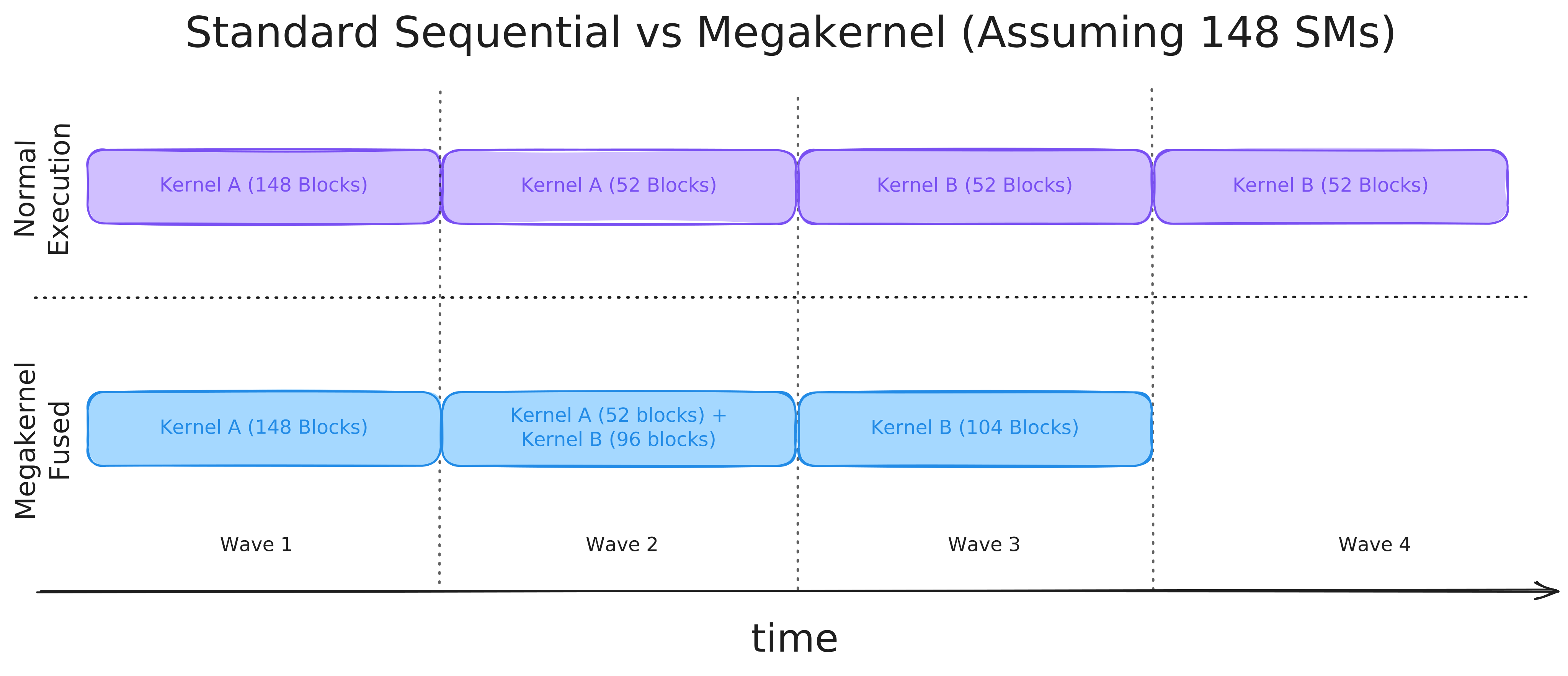
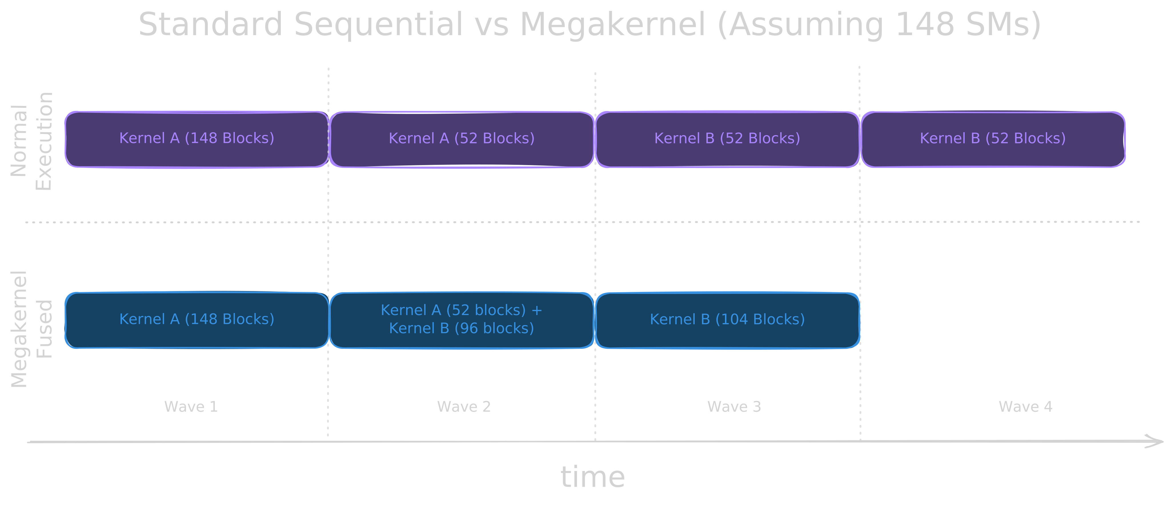
Assume you have two such kernels launched sequentially on the same cuda stream, both will have extra waves. Through some black magic, if we can combine the execution of both kernels, we can save a complete wave in theory and gain some free lunch.

Load/Store/Compute Overlap using TMA

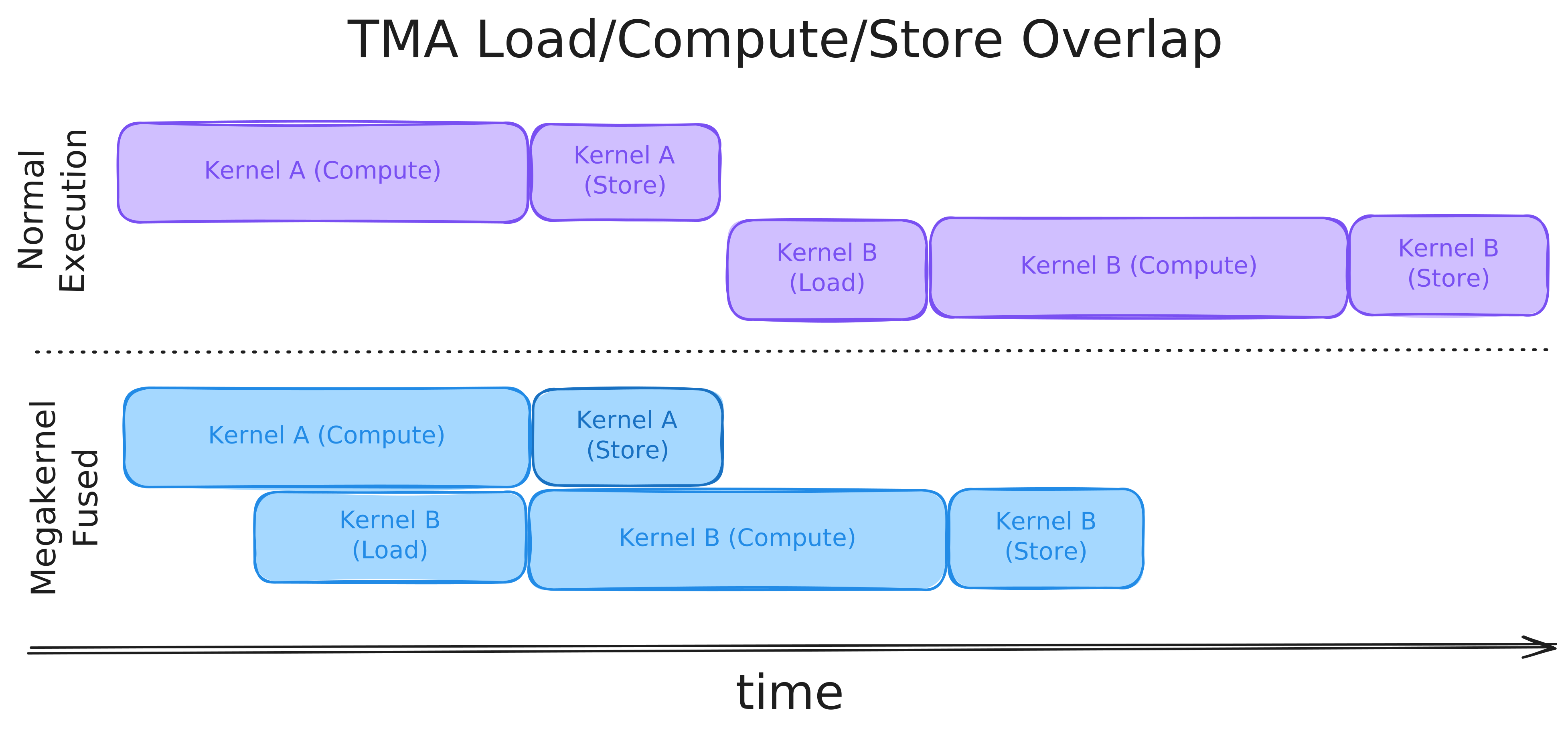
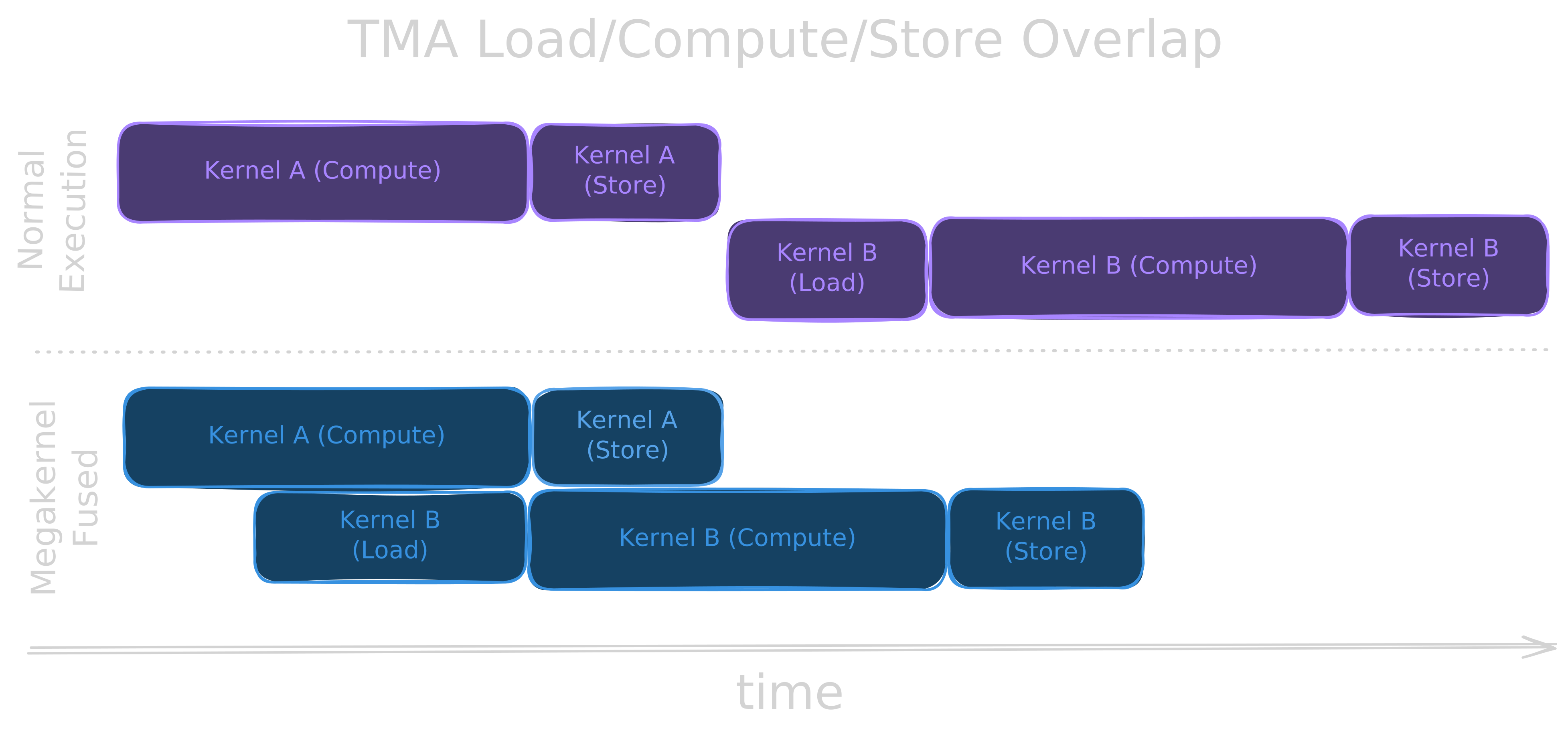
After scheduling properly, to squeeze out maximum performance, we can use TMA (Tensor Memory Accelerator) to asynchronously load the data required in the next wave while we are performing the computation of the current wave. Similarly, we can use TMA to perform asynchronous stores so that the next wave can run while the current store operation completes. This hides complete latency of load/store behind compute, similar to SoTA matmul kernels.

TMA Compute Overlap (Finegrained)

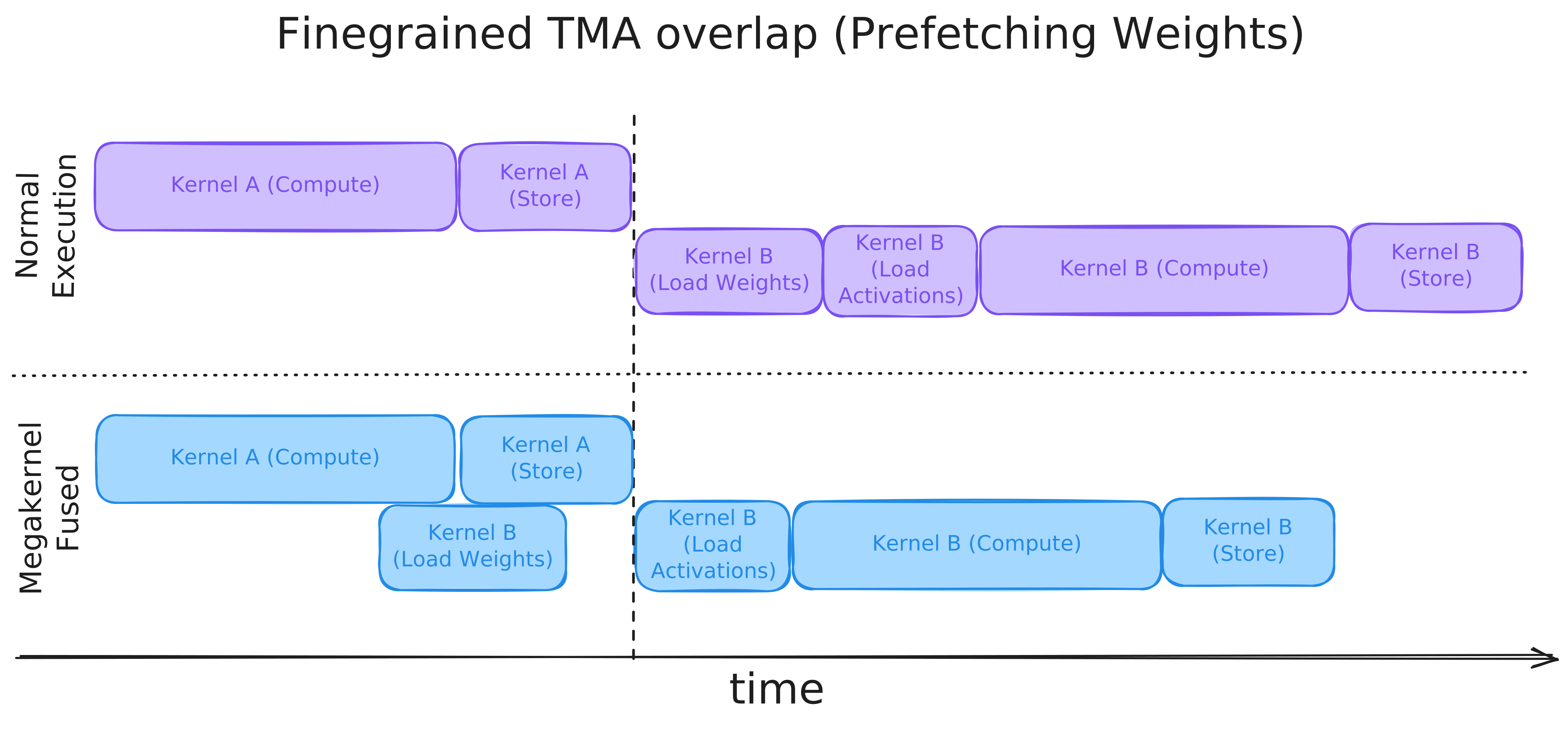
The above cases assume you don’t have data dependencies between kernels; otherwise, you cannot directly schedule them in parallel. Kernel B will require the output of Kernel A to be ready before it starts loading. But we are dealing with machine learning models that have weights + activations; we can still prefetch weights while the activations are not ready, overlapping load with compute.

Launch Overhead

A kernel launch is not as simple as it seems. The GPU has to set up context for the current kernel, clear the context of the previous kernel, flush the L1/L2 caches, etc. Although this takes a couple of microseconds, over 100s of passes, we can save a couple of milliseconds in total execution time.

By combining all of these strategies into a single megakernel, we bypass the standard GPU scheduler and minimize overhead. However, this means we must carefully build our own custom block scheduler directly into the kernel, manually managing data dependencies and synchronization across asynchronous execution blocks.

Implementation Plan

GPU Architecture

I have access to RTX 5070 Ti (sm120), so I decided to optimize for sm120 family of GPUs (RTX Pro 6000, RTX 50 Series, and DGX Spark). sm120 is the so-called “consumer blackwell”. It is an interesting architecture in the sense that it borrows hardware features from the Hopper family like TMA, and also has hardware support for block-scaled matrix multiplication (NVFP4, MXFP4, etc.), but uses warp-synchronous tensor cores unlike actual Blackwell (sm100 family), which has async tensor cores and TMEM (Tensor Memory). Apart from the above, there are a lot more differences we’ll encounter.

Model Architecture

• Currently focusing on a simple LLaMA-like (RMSNorm + SwiGLU) transformer architecture. As of now, I haven’t included RoPE and the final projection layer from embedding space to probabilities. I am currently focusing on the core components of the transformer, and will add the rest in future parts.
• This kernel isn’t for direct decode style inference, as we have to perform split-K GEMV and split-K attention (flash decoding) for efficient KV-Cache based decoding. Here I am doing a simple transformer forward pass with KV calculation (without any past KV cache) in a compute-bound regime, to showcase the performance benefits. These techniques can still be applied to single-batch decode kernels.

Why CuTe DSL?

The majority of DSLs operate on tile based abstraction, where we are only dealing with tile or vector-like data. To design a complex kernel with fine-grained hardware management, CuTe DSL is the way to go, as it gives Python flexibility while providing CUDA C++’s low-level control and compiling directly to PTX.

Megakernel Implementation

Cooperative Kernel

We launch the megakernel with gridSize == num SMs, allocating one block per SM. Each block acts like a CPU and decodes our custom instructions from global memory, where an instruction represents a unit of work containing an operator name (e.g., rmsnorm, matmul, attention) along with arguments and other metadata. We pre-schedule all instructions in order and assign the operator block to the actual kernel block. At runtime, each block reads its assigned instruction and executes the corresponding operator.

@cute.kernel
def kernel(max_works, mSchedule):
    block_idx = cute.arch.block_idx()[0]
    for work_idx in range(max_works):
        layer_idx    = mSchedule[block_id, work_idx, 0]
        op_kind      = mSchedule[block_id, work_idx, 1]
        pid_m        = mSchedule[block_id, work_idx, 2]
        pid_n        = mSchedule[block_id, work_idx, 3]
        pid_o        = mSchedule[block_id, work_idx, 4]
        expected_cnt = mSchedule[block_id, work_idx, 5]
        current_idx  = mSchedule[block_id, work_idx, 6]
        next_idx     = mSchedule[block_id, work_idx, 7]

        if op_kind == int(Op.RMS):
            ...
        elif op_kind == int(Op.QKV):
            ...
        elif op_kind == int(Op.ATTN):
            ...
        elif op_kind == int(Op.OUT):
            ...
        elif op_kind == int(Op.UP):
            ...
        elif op_kind == int(Op.GATE):
            ...
        elif op_kind == int(Op.DOWN):
            ...

Warpgroup Scheduling and Pipelineing

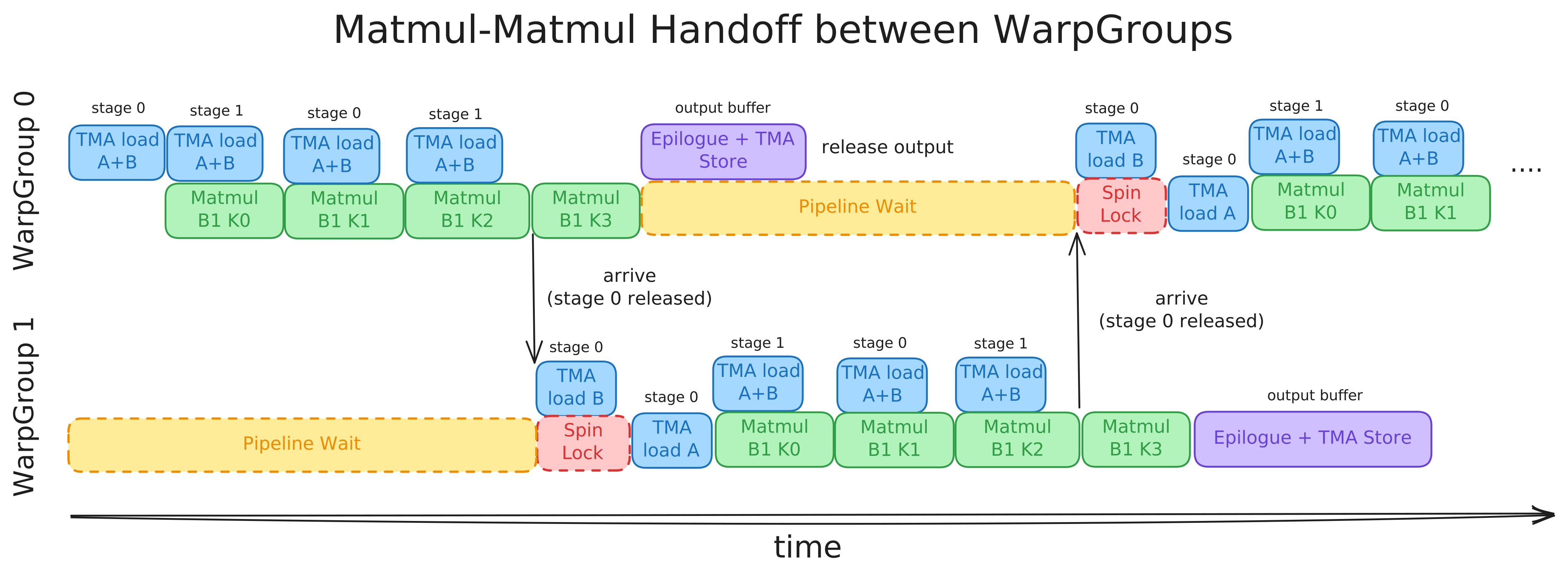
Each SM can run a maximum of 32 warps (1024 threads), but it can only schedule 4 warps (single warpgroup) at a time to the actual hardware. Taking that into consideration, we launch 2 warpgroups (= 8 warps) so that while one warpgroup (wg-1) is doing its computation, the other warpgroup (wg-2) can asynchronously load the data and wait for wg-1. As soon as wg-1 finishes, wg-2 starts its computation while wg-1 begins loading data for the next operation, similar to ping-pong matmul kernels.

# change the above code to this for double warpgroup - ping pong
@cute.kernel
def kernel(max_works, mSchedule):
    block_idx = cute.arch.block_idx()[0]
    warp_id   = cute.arch.warp_idx()
    group_id  = warp_id // 4

    for local_work_idx in range(max_works // 2):
        work_idx = local_work_idx * 2 + group_id
        ...

The async load/store handoff logic is written inside each operator. The entire architecture uses Ampere-style two-stage pipelining with TMA, two warpgroups operate in ping-pong fashion, and only one warpgroup is actively computing. At the same time, the other asynchronously loads data for the next operation. No warp specialization is used, both warpgroups are identical and simply alternate stages with proper barrier handoff and async stores.

I initially considered warp specialization because I frequently overflowed registers in the initial runs, and dedicating warps to producer/consumer roles would likely push us even further. That said, the kernel ended up using only 233 registers per thread. I’ll revisit warp specialization in the future.

Dependency Management and Scheduling

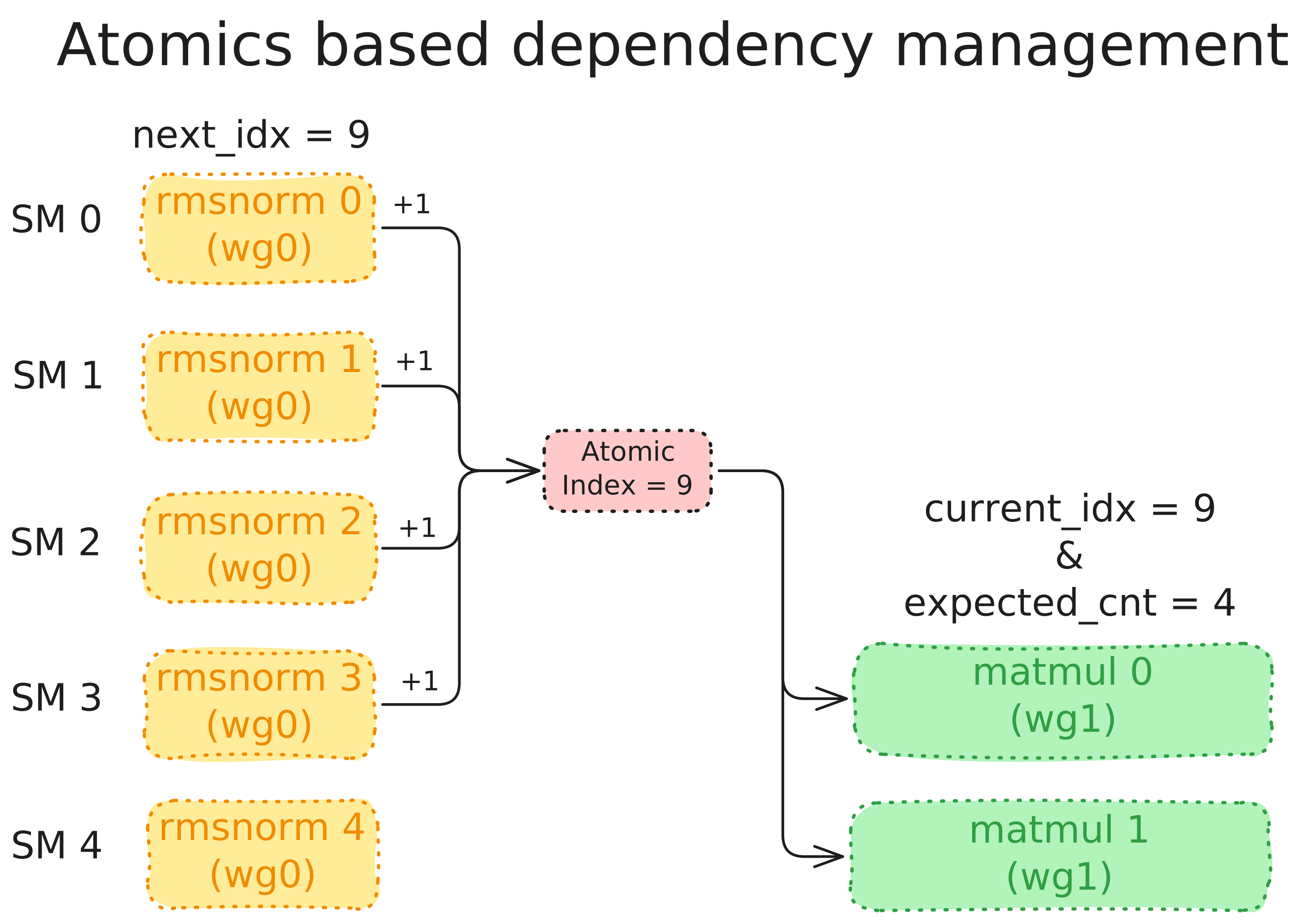
Scheduling is done in a simple round-robin manner across the SMs. For example, we have 8 RMS Norm blocks –> 12 Matmul blocks, and 8 Attention blocks to be scheduled on 5 SMs. We would create the mSchedule to follow the diagram below.

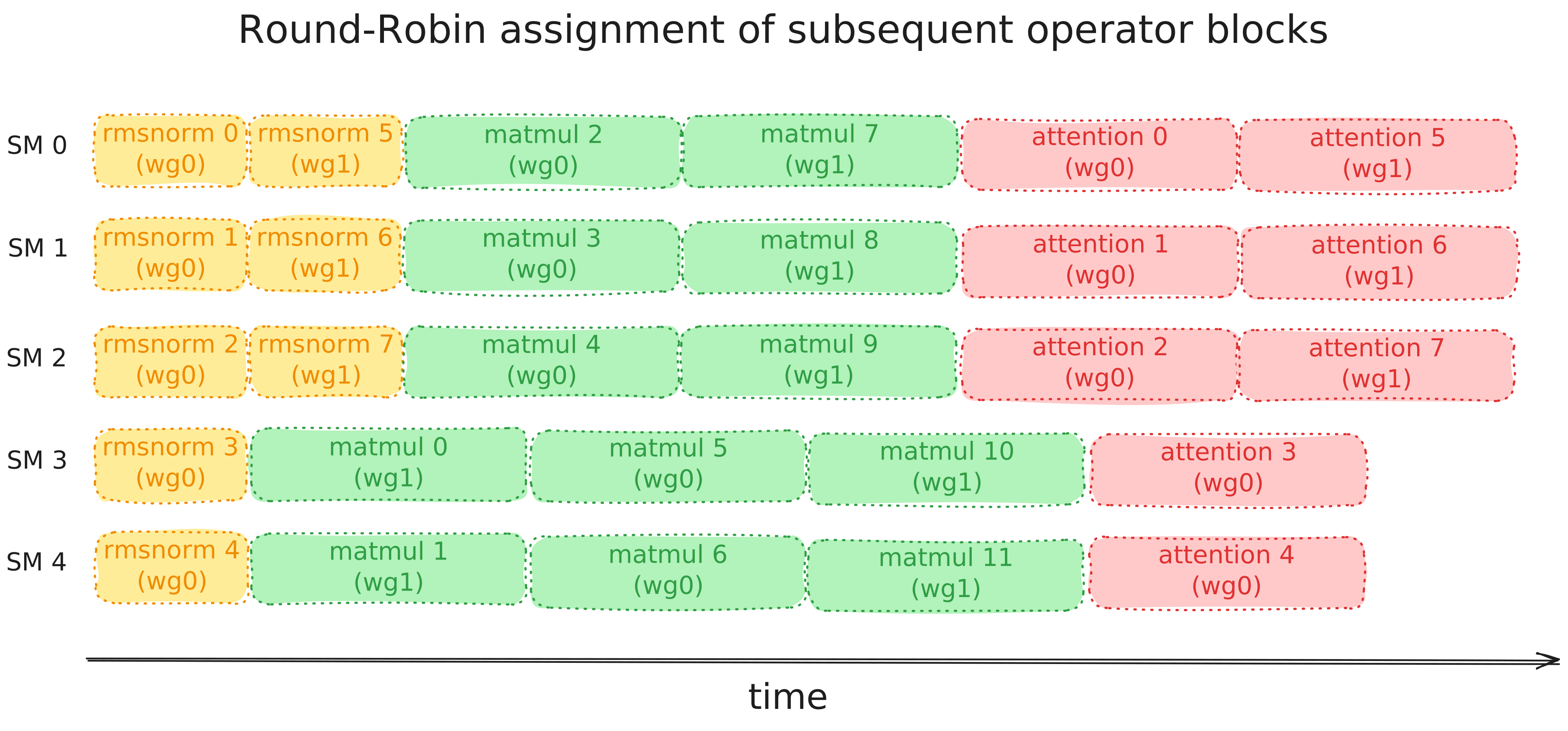
This eliminates wave quantization bubbles and the double warpgroup ping-pong eliminates load/store bubbles. But we cannot directly schedule blocks we have to make sure that the previous output is ready.

The inter-block dependencies are managed using an atomic spin-lock. For each block, we identify all its parent dependencies. When a parent block finishes its computation, it increments an atomic counter at its next_idx by 1. The current block polls the counter at current_idx and as soon as it reaches the predetermined value expected_cnt, it begins execution.

Shared Memory Layout

The sm120 architecture provides 99 KiB of max usable shared memory per SM. To ensure smooth, non-blocking handoff between operators, the shared memory is statically partitioned into three regions:

I have adopted a static shared memory layout. You can refer to megakernel blog by Hazy Research [3], which implements a page-based shared memory allocator with 16 KiB pages allocated at runtime. But in my case, static might be simple with two stages instead of adding an extra allocator. Initially, I had tried with three stages, but that limited the size of matmul stages and reduced performance for large matmuls, so I reverted to two stages.

@cute.jit
def _get_shared_storage(self):
    num_out_elements = max(
        self.bM * (self.bN + self.output_pad),
        self.bQ * (self.head_dim + self.output_pad),
        self.num_sets * self.embed_dim * self.num_stages,
    )

    @cute.struct
    class BarrierStorage:
        load_barrier:    cute.struct.MemRange[Uint64, self.num_stages]
        input_barrier:   cute.struct.MemRange[Uint64, 2]
        output_barrier:  cute.struct.MemRange[Uint64, 2]
        compute_barrier: cute.struct.MemRange[Uint64, 2]
        stage:           cute.struct.MemRange[Int32, 1]
        phase:           cute.struct.MemRange[Int32, 1]

    @cute.struct
    class SharedStorage:
        barriers: BarrierStorage
        stages: cute.struct.Align[cute.struct.MemRange[BFloat16, self.num_stages*self.stage_elements], 128]
        out:    cute.struct.Align[cute.struct.MemRange[BFloat16,num_out_elements], 128]

    return SharedStorage

def kernel(...):
    storage = self._get_shared_storage()

While one warpgroup computes using stage0, the other prefetches into stage1. On the next iteration they swap, this is the classic ping-pong pattern extended uniformly across all operators. Each operator’s input tiles must fit within the 32 KiB upper limit of a single-stage buffer. But operations like matmul use both stages even though a single warpgroup is running that operation. Near the end of the operation, it ensures that the other warpgroup starts with the freed stage, so we pipeline both at the inter-op and intra-op levels.

Note that sm120 does not support TMA Swizzled Stores, unlike the sm100 architecture, so we add 16 bytes of padding per row to the output tiles stored in shared memory to prevent bank conflicts during the store phase.

• Matmul: Each stage holds both the A and B tiles in fp16. With $\mathrm{blockM} = 64$, $\mathrm{blockN} = 128$, and $\mathrm{blockK} = 64$:

The matrix multiply accumulates in float32 registers but the result is cast back to fp16 before being written to shared memory, so the output footprint uses 2 bytes per element rather than 4. With 16-byte row padding:

• Attention: I have used Flash Attention v2’s approach, where each stage holds the Q, K, and V tiles. With $\mathrm{blockQ} = 64$, $d_{\mathrm{head}} = 128$, and $\mathrm{blockKV} = 64$ in fp16, each tile occupies:

However, Q and V are aliased in shared memory. Q is loaded once at the start of the attention loop using cp.async / LDGSTS instruction and is completely loaded into registers after that, so its buffer is reused for V during the K/V streaming phase. At any point during the loop, a single stage holds:

The attention output with row padding:

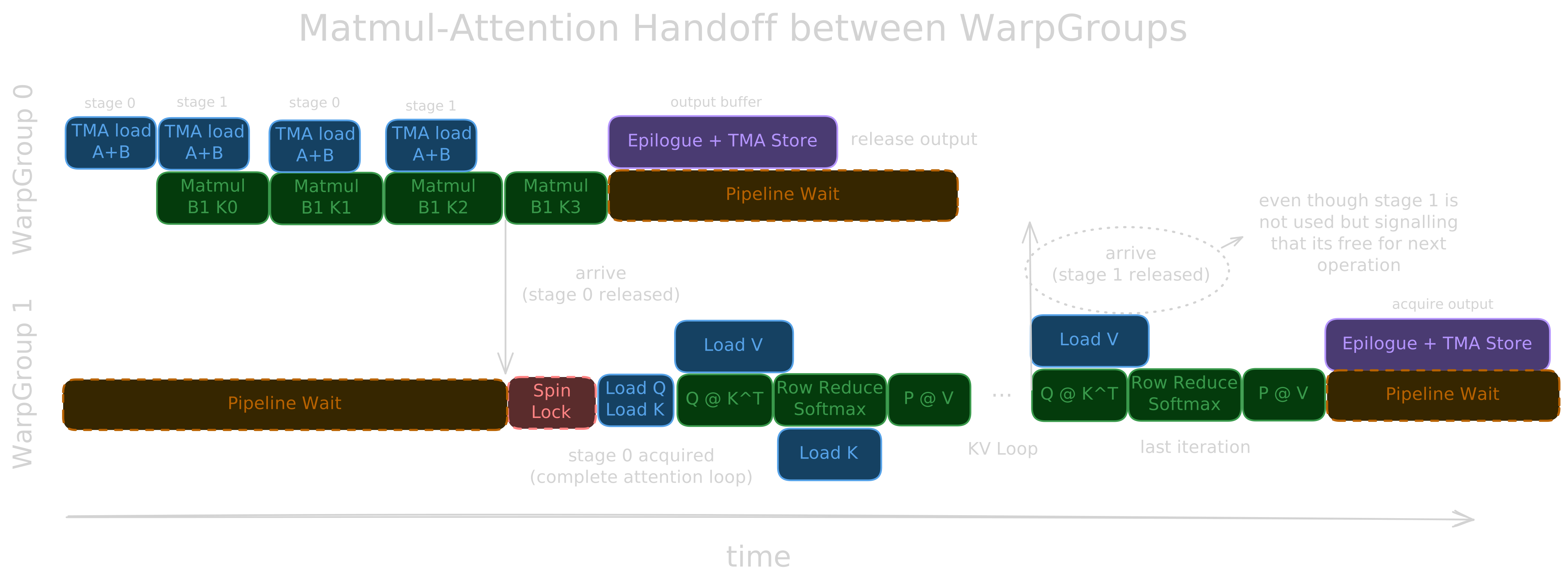
The attention kernel itself is not multi-stage; the KV loop operates within a single-stage buffer, but overlaps memory and compute by loading V. At the same time, the Q @ K^T matmul executes while loading the next K tile, and the P @ V matmul executes. The two-stage ping-pong only applies across operators: once attention finishes, the next operation begins on the other stage.

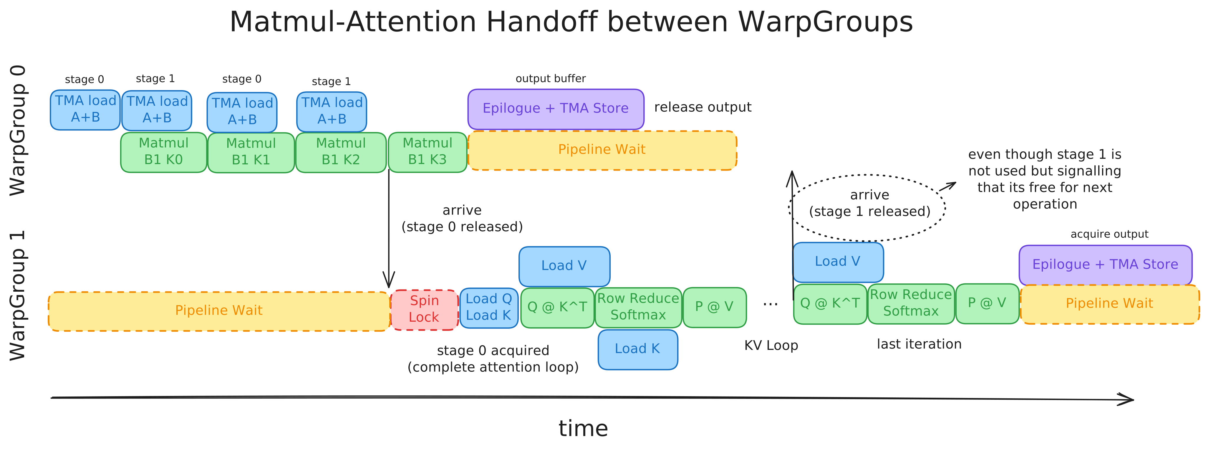
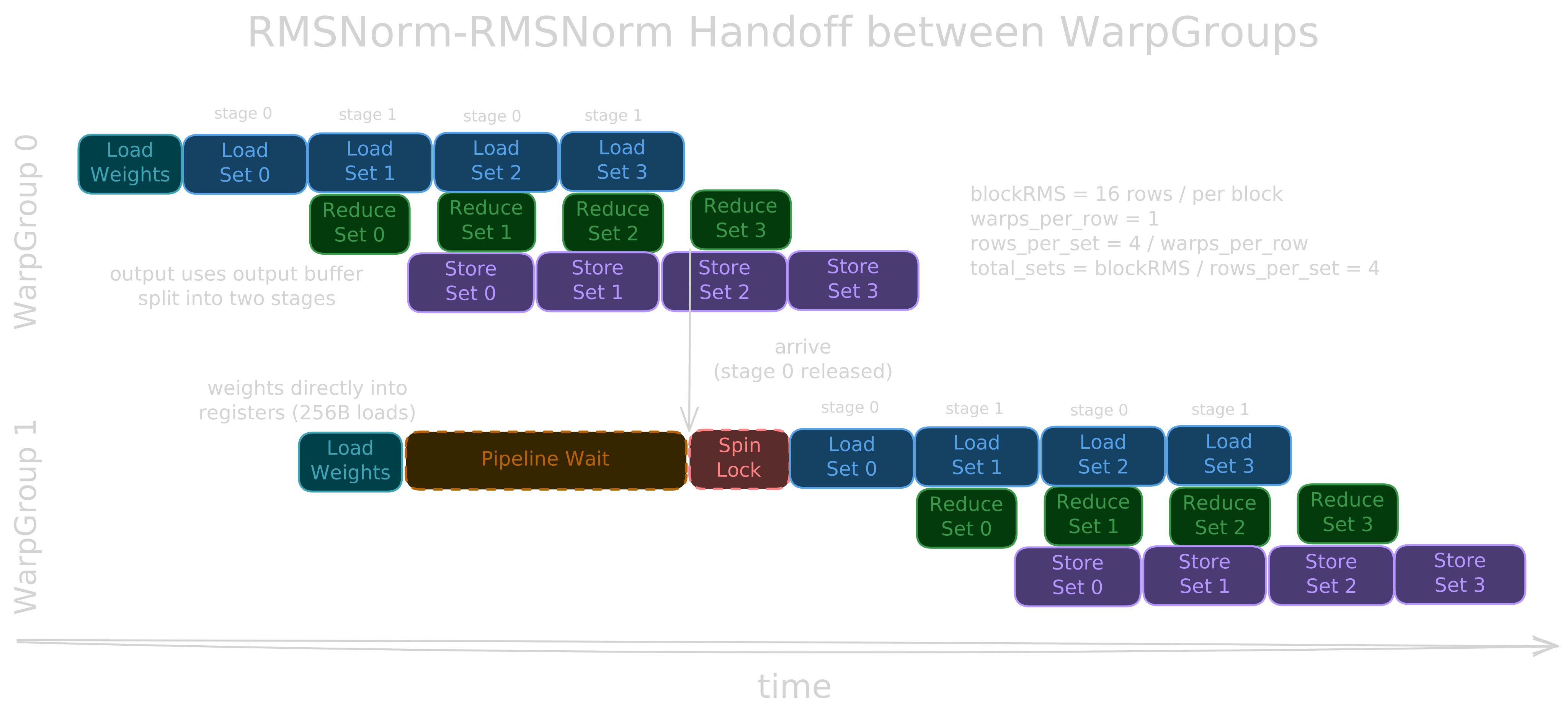
• RMSNorm: The row-parallel work distribution is designed to maximize strong scaling across SMs. For N rows, each block is assigned prev_power_of_two(N / num_sms) rows to ensure even work distribution. Within each block, a warps_per_row parameter controls how many of the 4 available warps cooperate to normalize a single row; for instance, warps_per_row = 2 means two rows are computed simultaneously, each processed by 2 warps. These rows are again two-stage pipelined, one set of rows is being normalized, while the next set is being loaded asynchronously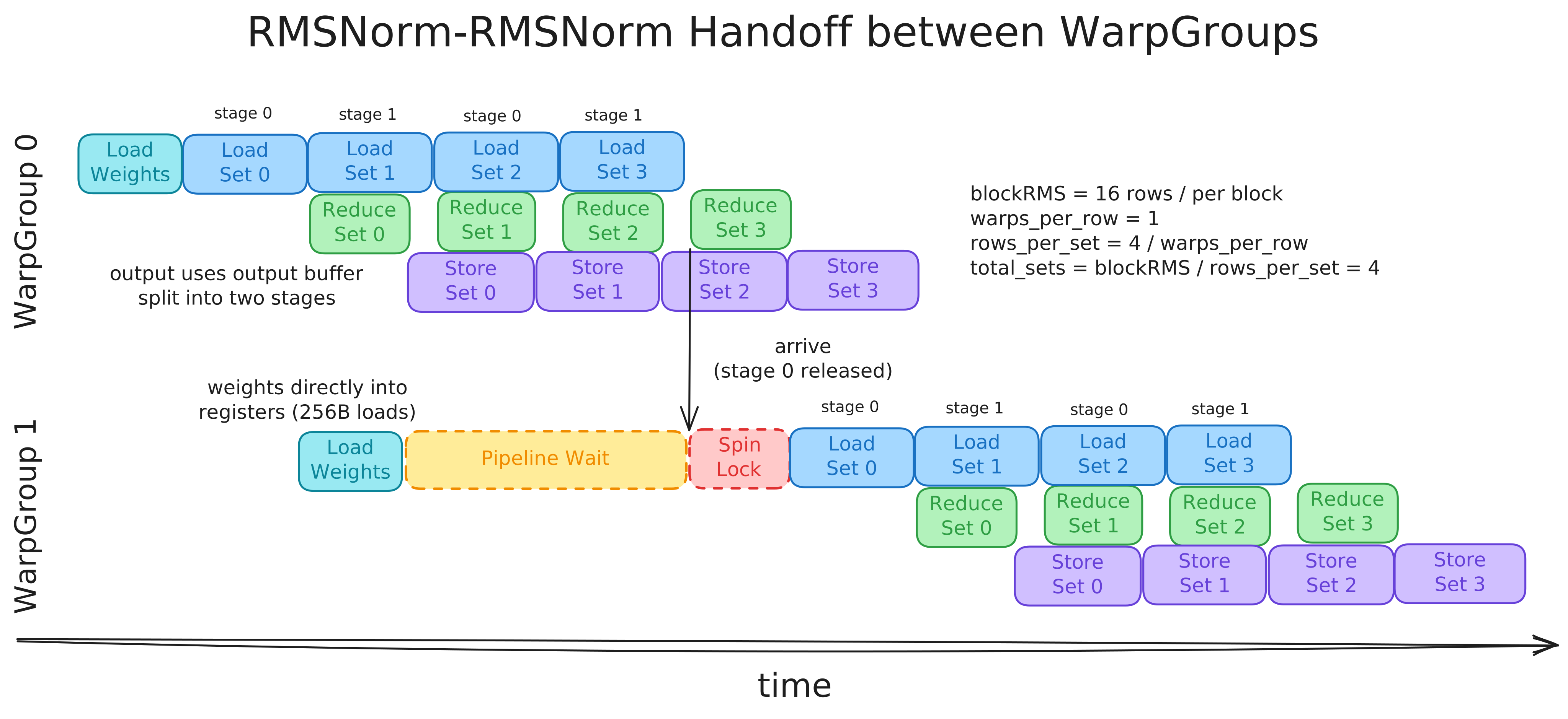

  

Synchronization

To manage such pipelines there are three barriers, namely input_barrier, compute_barrier and output_barrier per warpgroup and an additional set of load_barrier one for each stage. We have 2x3 + 1x2 = 8 barriers, all of them are mbarrier where threads can arrive, wait for other threads or wait for memory transactions.

As there are barriers for each warpgroup I have named them input_bar_me (current warpgroup) and input_bar_ot (other warpgroup). The same scheme applies to output_barrier and compute_barrier.

• input_barrier: Sits at the very start of the operator. We wait on the barrier (input_bar_me) until the other warpgroup arrives on its input_bar_ot. It signals the warpgroup that the input stage has been released and is now ready to start loading data. After the barrier, there is a load_stage variable in shared memory that indicates the stage to be used in the current iteration. The other warpgroup updates it before arrival on input_bar_ot.

• compute_barrier: input_barrier only guarantees that one of the stage buffers is released but not both. Therefore another barrier is required to signal that all stages are now released and we can start computing on the released stage. This barrier is placed just before loading the next pipeline stage.

• output_barrier: output_barrier guarentees that the output buffer is released so the wait(output_bar_me) is placed jut before writing anything to the output buffer and arrive(output_bar_ot) is placed after the output is fully stored from SMEM to GMEM.

Atomic Spin Lock

Just after the input_barrier a single thread spins on the current_idx of the atomic array untill its value reaches expected_cnt.

@dataclass
class PipelineMeta:
    current_idx: int
    next_idx: int
    expected_cnt: int

if group_tid == 0: #group_tid = local thread index of the warpgroup
    ready = 0
    while ready != pipeline.expected_cnt:
        ready = ld_acquire_u32((mAtomics.iterator + pipeline.current_idx).toint())
    warpgroup_sync()

These are the main concepts used in the kernel, after this the remaining part is working with CuTe DSL to actually implement the code, profiling kernels and benchmarking. I did not arrive at this architecture directly, it took multiple iterations, errors, and race conditions that needed to be fixed. I’ll explain those nuances in the code section.

Implementation in CuTe DSL

In CuTe DSL, you have to wrap the Python functions with @cute.jit and @cute.kernel. @cute.jit has the code which is going to get JIT compiled, it can be either a CPU/GPU function. @cute.kernel is the actual entry point of the kernel which is launched with .launch(grid=(num_sms,), block=(256,)) method of the wrapper.

Load / Store Ops

LDGSTS and Register Copies

There are multiple ways you can load / store date from registers to Global and Shared memory. https://yang-yifan.github.io/blogs/cute_copy/cute_copy.html has a great blog with different ways to copy the data. To use the LDGSTS async copy (introduced in Ampere for async GMEM <-> SMEM copies) you have to use cute.make_tiled_copy with cpasync.CopyG2SOp, below is the implementation in the attention operator.

def get_tiled_copy_cpasync(self) -> cute.TiledCopy:
    atom_async = cute.make_copy_atom(
        cpasync.CopyG2SOp(cache_mode = cute.nvgpu.LoadCacheMode.GLOBAL),
        cutlass.BFloat16, num_bits_per_copy = 128
    )
    async_elems     = 128 // 16
    cols_per_pass   = self.config.head_dim // async_elems
    rows_per_pass   = 128 // cols_per_pass
    tKV_layout      = cute.make_ordered_layout((rows_per_pass, cols_per_pass), order=(1, 0))
    vKV_layout      = cute.make_layout((1, async_elems))
    gmem_tiled_copy = cute.make_tiled_copy_tv(atom_async, tKV_layout, vKV_layout)
    return gmem_tiled_copy

There is also cute.autovec_copy where you have to give the thread partitions of any of RMEM / GMEM / SMEM and cute will use the most efficient copies for the same. The weights are loaded from GMEM to RMEM using cute.autovec_copy.

TMA Copies

I have used TMA for all tensor load / store operations except for weights of RMSNorm (direct register copy) and Attention (LDGSTS). Given N transformer layers the make the weights of each operator stacked contigously in memory, so a weight matrix of shape (A, B) is now shaped (N, A, B). This allows use to use a single TMA descriptor for the weights of multiple layers, by adding an extra dim in TMA.

Then create shared memory layouts for the tensors (they should have the exact dimensions and strides of a single tile). For padded stores using TMA, we create a shared memory layout with a larger shape than the global gC_tile. The TMA hardware then automatically clips the output tile and doesn’t write those extra bytes. The normal sC_layout does not work with TMA if you want to clip the dims.

## TMA Layouts given while creating TMA atoms

sA_layout = cute.make_composed_layout(
    cute.make_swizzle(int(math.log2(bK)) - 3, 4, 3), 0,
    cute.make_ordered_layout(
        shape = (bM, bK),
        order = (1, 0)
    ),
)

sB_layout = cute.make_composed_layout(
    cute.make_swizzle(int(math.log2(bK)) - 3, 4, 3), 0,
    cute.make_ordered_layout(
        shape = (1, bN, bK),
        order = (2, 1, 0)
    ),
)

sC_layout = cute.make_layout(
    shape = (bM, bN),
    stride = (bN + pad, 1) #pad = 8 elements = 16 bytes
)

# Same as the above sC_layout but with contiguous strides
# Matmul output tensors have this layout where the last dim is split in bN blocks
# this allows TMA to clip the padding bytes, therefore we have to add an extra dimension in the sC_tma layout
# cute.make_ordered_layout(
#     shape = (self.num_tokens, self.ff_dim // self.bN, self.bN),
#     order = (2, 1, 0),
# )
sC_tma_layout = cute.make_ordered_layout(
    shape = (bM, 1, bN + output_pad), order = (2, 1, 0),
)

TMA atoms are created before the kernel inside the __call__ function for the input, weights, and output activations involved in each of the operations. The atoms already have the TMA descriptors embedded in them, we don’t have to create them separately. For matmul operations where the activations have pointwise addition in the epilogue, we can use the in-place reduction feature while performing TMA Stores.

load_op  = cpasync.CopyBulkTensorTileG2SOp()
store_op = cpasync.CopyBulkTensorTileS2GOp()
if cutlass.const_expr(self.use_tma_reduce):
    store_op_red = cpasync.CopyReduceBulkTensorTileS2GOp(cute.ReductionKind.ADD) #cp.async.reduce.bulk.tensor.3d...
else:
    store_op_red = store_op

# QKV (WS1 @ QKV_w -> WS2)
tma_QKV_inp, g_QKV_inp = cpasync.make_tiled_tma_atom(load_op,  mWS1_embed, sA_layout,  (bM, bK))
tma_QKV_wt,  g_QKV_wt  = cpasync.make_tiled_tma_atom(load_op,  mQKV_proj,  sB_layout,  (1, bN, bK))
tma_QKV_act, g_QKV_act = cpasync.make_tiled_tma_atom(store_op, mQKV_act,   sC_tma_layout, (bM, 1, bN + output_pad))
... #similarly for all operation

We cannot pass the raw mWS1_embed tensor in the TMA’s runtime code, we have to pass the tensor returned in the code above because it is a special ArithmeticTuple tensor with vectorized strides, allowing us to slice into the tile of the global tensor. During runtime, within the matmul() function, the code snippet below creates per-thread partitions for the TMA operation.

## in matmul.py during runtime
# Actually layout with stages and a stride of 32 KiB between stages
sA_layout = cute.make_layout(
    shape = (bM, bK, num_stages),
    stride = (bK, 1, stage_elements)
)
sB_layout = cute.make_layout(
    shape = (bN, bK, num_stages),
    stride = (bK, 1, stage_elements)
)
sC_layout = cute.make_layout(
    shape = (bM, bN),
    stride = (bN + output_pad, 1)
)
sC_tma_layout = cute.make_layout(
    shape = (bM, bN + output_pad),
    stride = (bN + output_pad, 1)
)

swizzle = cute.make_swizzle(3, 4, 3) # for K = 128

stages_ptr = storage.stages.data_ptr()
sA = cute.make_tensor(cute.recast_ptr(stages_ptr, swizzle), sA_layout)
sB = cute.make_tensor(cute.recast_ptr(stages_ptr + bM * bK, swizzle), sB_layout)

sC_tma = storage.out.get_tensor(sC_tma_layout)

sA_g = cute.group_modes(sA, 0, 2) # (bM, bK, num_stages) -> ((bM, bK), num_stages)
sB_g = cute.group_modes(sB, 0, 2) # (bN, bK, num_stages) -> ((bN, bK), num_stages)
gA_g = cute.group_modes(gA_tile, 0, 2) # (bM, bK) -> ((bM, bK), )
gB_g = cute.group_modes(gB_tile, 0, 3) # (1, bN, bK) -> ((1, bN, bK), )

tAsA, tAgA = cpasync.tma_partition(tma_A, 0, cute.make_layout(1), sA_g, gA_g) # per thread view of sA and gA
tBsB, tBgB = cpasync.tma_partition(tma_B, 0, cute.make_layout(1), sB_g, gB_g) # per thread view of sB and gB

We have to group the tile-shape mode for TMA to interpret the exact tile, and the rest of the modes can be used as stages for async copies. TMA copies are called using cp.async.bulk.tensor.2d. ... instruction which is to be called by a single thread asynchronously and pass tile coordinates, descriptor pointer and destination address to the instruction. Same thing is done by cute.copy(...) function below. cute.copy(...) with TMA atom internally calls cute.elect_one() which elects a single thread from a warp to run that instruction therefore we have to wrap it in if warp_id == 0:, if you pass cute.copy(...) in elect_one() then it will stall execution because of calling nested elect_one(), this is a common pitfall to avoid.

Leading box dimention in TMA cannot exceed 256, if it exceeds, CuTe compiler automatically folds the dimention by adding extra dim fox example (512, 64) -> (256, 2, 64) but in my case it produced very inefficient code and also created TMA copies at unalligned memory addresses, so manually folding the dim into something <= 256 is recommended.

if warp_id == 0:
    with cute.arch.elect_one():
        cute.arch.mbarrier_arrive_and_expect_tx(load_barrier + stage_idx, 2) # increment transcation count
    cute.copy(tma_A, tAgA[None, tile_idx], tAsA[None, stage_idx], tma_bar_ptr = load_bar + stage_idx)

For TMA stores, we have to perform the same operations groupmodes -> partition -> copy, but TMA stores don’t support the mbarrier completion mechanism; therefore, we also have to call the bulk_group API to commit the store and track it. Additionally, I have called fence_proxy_async_global() to ensure that stores are visible to other SMs. Without this, you will constantly have race conditions within SMs. It took Claude and me a while to figure this out.

if warpgroup.warp_id == 0:
    gC_tma_tile = cute.local_tile(gC_tma, (bM, 1, bN + output_pad), (pid_m, pid_n, 0))
    sC_g     = cute.group_modes(sC_tma,      0, cute.rank(sC_tma.layout))
    gC_tma_g = cute.group_modes(gC_tma_tile, 0, cute.rank(gC_tma_tile.layout))
    sC_part, gC_part = cpasync.tma_partition(tma_C, 0, cute.make_layout(1), sC_g, gC_tma_g)
    cute.copy(tma_C, sC_part, gC_part)
    cute.arch.cp_async_bulk_commit_group()
    cute.arch.cp_async_bulk_wait_group(0)
    fence_proxy_async_global()

LdMatrix / StMatrix Instructions

These copies are similar to most of the copy atoms, but you have to be careful when to use transpose, when not to use transpose, and the data type. CuTe DSL actually simplifies the usage of this API by handling address generation and applying swizzling automatically, or else it was a huge pain to use ldmatrix and stmatrix instructions with inline ptx.

# group_tidx is thread index within a warp group
tiled_mma = cute.make_tiled_mma(
    warp.MmaF16BF16Op(BFloat16, Float32, (16, 8, 16)),
    (warpM, warpN, 1), permutation_mnk = (bM, bN, bK),
)

thr_mma = tiled_mma.get_slice(warpgroup.group_tidx)

# This seems confusing, but it creates register tensors based on per-thread partitioned shared memory
tCrA = thr_mma.make_fragment_A(thr_mma.partition_A(sA[None, None, 0]))
tCrB = thr_mma.make_fragment_B(thr_mma.partition_B(sB[None, None, 0]))

ldmatrix = cute.make_copy_atom(warp.LdMatrix8x8x16bOp(transpose=False, num_matrices=4), BFloat16)
thr_copy_A = cute.make_tiled_copy_A(ldmatrix, tiled_mma).get_slice(warpgroup.group_tidx)
thr_copy_B = cute.make_tiled_copy_B(ldmatrix, tiled_mma).get_slice(warpgroup.group_tidx)

tCsA = thr_copy_A.partition_S(sA[None, None, stage_idx])
tCsB = thr_copy_B.partition_S(sB[None, None, stage_idx])

# reshape according to ldmatrix (only for copy)
tCrA_cpy = thr_copy_A.retile(tCrA)
tCrB_cpy = thr_copy_B.retile(tCrB)

cute.copy(thr_copy_A, tCsA, tCrA_cpy)
cute.copy(thr_copy_B, tCsB, tCrB_cpy)

cute.gemm(tiled_mma, tCrC, tCrA, tCrB, tCrC)

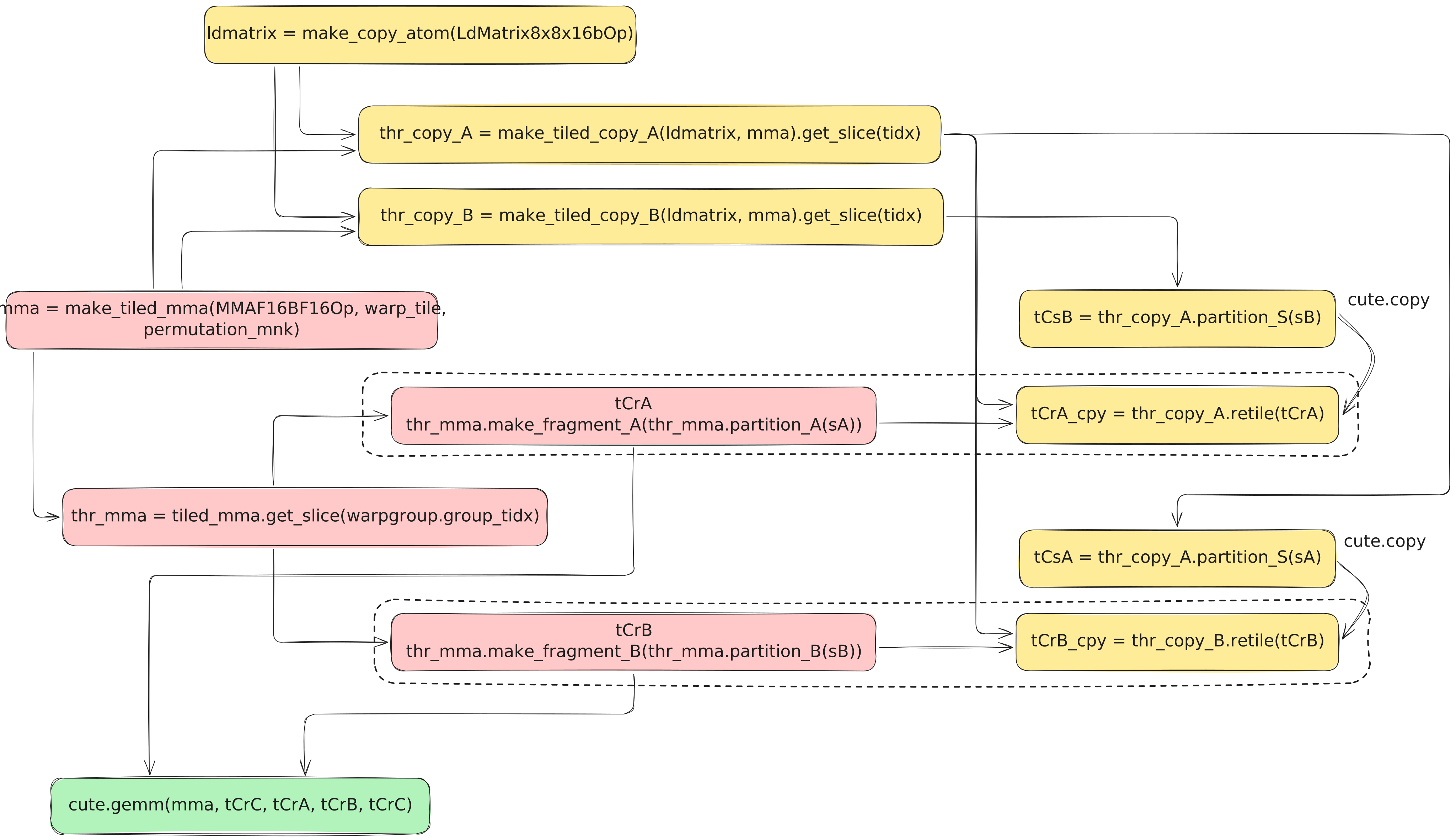
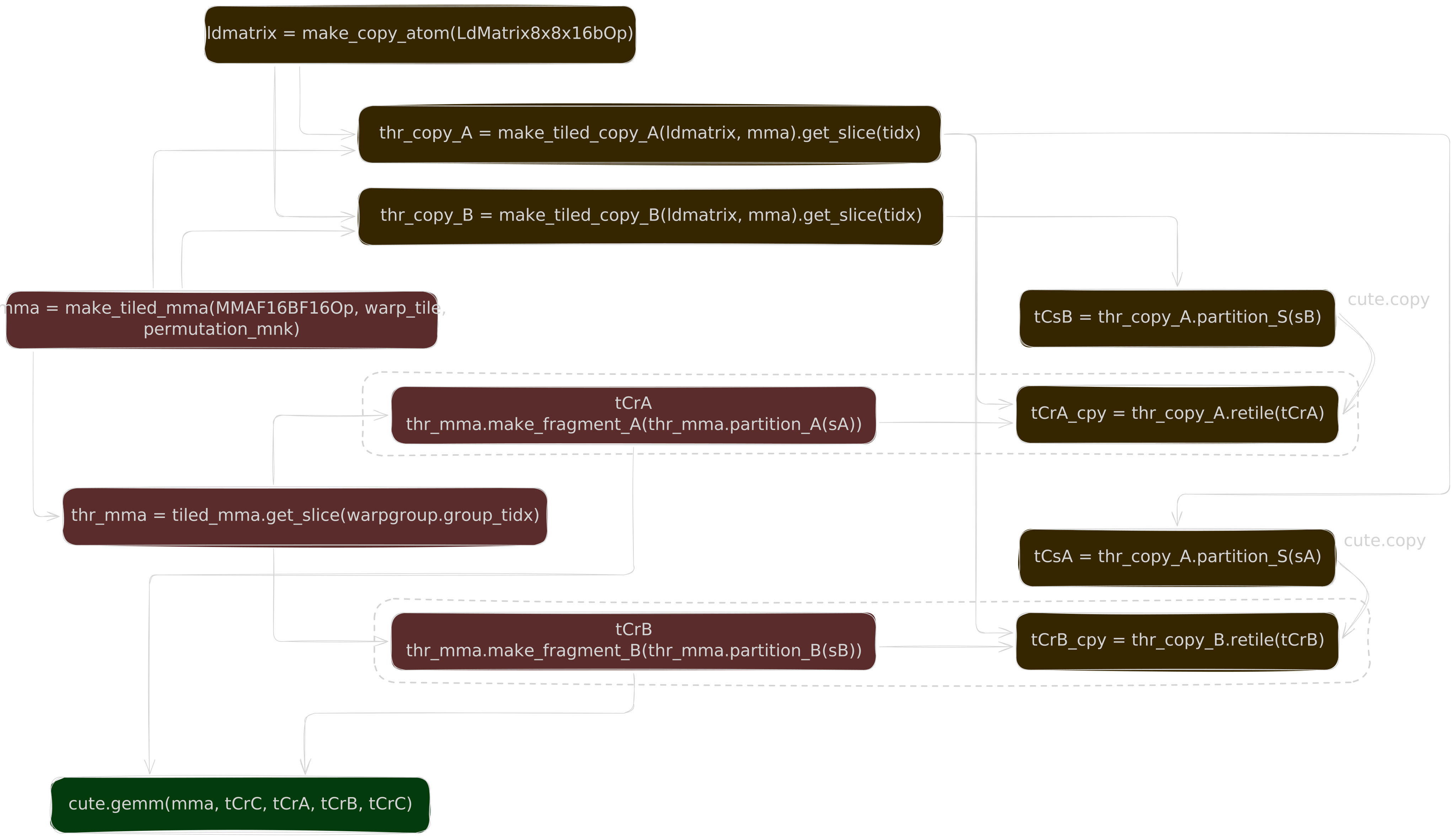
Similarly, for storing, we have to use stmatrix atom and cute.make_tiled_copy_C, and the rest is similar.

thr_mma = tiled_mma.get_slice(warpgroup.group_tidx)
store_atom = cute.make_copy_atom(
 cute.nvgpu.warp.StMatrix8x8x16bOp(num_matrices=4), cutlass.BFloat16
)
thr_copy_C = cute.make_tiled_copy_C(stmatrix, tiled_mma).get_slice(warpgroup.group_tidx)

TensorSSA

Ideally, you cannot do any vectorized operations on any of cute.Tensor, to ease out vector operations, you can call .load() on cute.Tensors which returns a TensorSSA object. TensorSSA is a vectorized IR of the underlying tensor, you can perform broadcasting, reductions (both local and warp) and pointwise operations on that object with self and other TensorSSA objects. Finally, you can call .store(result) on the cute.Tensor where you want to store the result, and the compiler will automatically generate code for it. This is the attention row-reduction in TensorSSA:

scores_mn = Attention._reshape_acc_to_mn(acc_S)
output_mn = Attention._reshape_acc_to_mn(acc_O)

for r in cutlass.range_constexpr(num_rows_per_thr):
    scores      = scores_mn[r, None].load()
    prev_max    = row_max[r]
    block_max   = scores.reduce(cute.ReductionOp.MAX, prev_max, 0)
    block_max   = cute.arch.warp_reduction_max(block_max, threads_in_group=4)
    row_max[r]  = block_max
    safe_max    = block_max if block_max != -Float32.inf else 0.0

      # use fastmath to utilize SFU on GPUs
    probs       = cute.math.exp2(
    (scores - safe_max) * softmax_scale_log2, fastmath = True)
    rescale     = cute.math.exp2(
    (prev_max - safe_max) * softmax_scale_log2, fastmath = True)

    output_mn[r, None].store(output_mn[r, None].load() * rescale)
    row_sum[r]  = probs.reduce(cute.ReductionOp.ADD, row_sum[r] * rescale, 0)
    scores_mn[r, None].store(probs)

Matmul Instructions

Currently this is a simple explanation of warp sync tensor cores APIs, will cover tcgen05 sometime in future. The pattern is similar first create an MMAOp then create a TiledMMA using cute.make_tiled_mma(...). TiledMMA can be called directly with cute.gemm, using the per-thread register partitions as arguments. It is also used to create TiledCopy for LdMatrix / StMatrix operations.

from cutlass import BFloat16, Float32
from cutlass.cute import warp

cute.make_tiled_mma(
    warp.MmaF16BF16Op(BFloat16, Float32, (16, 8, 16)),
    (warpM, warpN, 1), permutation_mnk = (bQ, bKV, head_dim),
)

(warpM, warpN, 1) are warp tiling dimensions, which means there will be warpM warps in the M dimension and warpN warps in the N dimension. Then there is permutation_mnk, which is the complete tile size on which this MMA Op will work. To make things clear assume permutation_mnk is (128, 128, 64) so all involved warps will work on this massive tile, and a warp tiling of (2, 2, 1) means each warp will work on 64 cols and 64 rows. BUT this is just the tip of the iceberg, you can do far more complex things with permutation_mnk, it accepts cute.layout in each dimension where you can specify how those 64 rows and 64 cols will be arranged. You can refer to this GitHub issue for more information on permutation_mnk.

Profiling

Profiling is where most of the kernel-development time goes. Modal does not support profiling with nsight-compute, so I used Lightning AI. Before profiling, compile the CuTe DSL kernels with os.environ["CUTEDSL_EXPORT_LINEINFO"] = "1" to preserve the source mappings for SASS and PTX. In the source view, place the source on the left and the PTX on the right.

Bank Conflicts

There are already great posts on bank conflicts if you are new to this topic, and it is a prerequisite before moving ahead. For the matmul operands, bank conflicts are removed by applying Swizzle<3, 4, 3> layout to input tensors, which applies a 128B swizzle with 16B granularity and is supported by TMA for in-flight swizzle. The output tensor from matmul has an extra 16B of padding to prevent bank conflicts during storage. Similarly, for attention the Swizzle<3, 3, 3> pattern is applied since blockKV and blockQ are as of now hardcoded to 64. To identify bank conflicts in Nsight Compute, use PM Sampling (Ampere+) in the L1 Hit Miss section to inspect the distribution of bank conflicts across the kernel timeline.

Recent versions of Nsight Compute also include the Function Stats Window. Select the timeline region where conflicts occur, and the window highlights the source lines responsible for most of the instructions in that region. You can jump to those instructions, or open the Source tab and look for code where L1 Shared Excessive Wavefronts exceeds 0%, which directly indicates bank conflicts.

Additional things to look for

• Make sure to use 256B loads/stores which were added in sm120 and sm100 architectures.
• In the atomic spin-lock polling loop, ptxas automatically introduced a yield instruction. It deprioritizes the current warp as soon as it hits the yield instruction because the compiler automatically determines that it should not waste resources on the spin lock counter.
• Inspect both compute and memory throughput. Very high memory throughput can indicate poor L2-cache reuse or memory-bound operation which is why state-of-the-art matmul kernels use L2-cache-aware tiling. This kernel is compute-bound, so increased compute throughput directly improves performance.
• Avoid register spills. Spilled registers are stored in local memory, which resides in DRAM and can severely bottleneck execution. Although PTX 9.0 provides an option to spill registers to shared memory, avoiding spills is still preferable. For example, directly loading the other tensor from global memory into registers in the SiLU epilogue caused excessive spilling therefore I manually introduced a minibatch instead of loading the complete tile all at once. In the SASS view, search for LDL and STL instructions to see exactly where the registers are spilled.
• A high L2 Theoretical Sectors Global Excessive value on the Details page indicates that global loads are not coalesced efficiently. Improve the access pattern to use the available memory bandwidth more effectively. (permutation_mnk layouts can be used in matmul atoms for to store matmul outputs in contiguous format which can decrease this metric)
• Use Warp State Statistics to understand the average state of each warp. In this kernel, four of eight warps are intentionally sleeping, so a spike in Stall Sleeping is expected. Ignore that expected behavior and focus on Stall Math Pipe Throttle, which means the warps are waiting on compute instructions a positive sign here because the tensor and CuTe cores are heavily utilized. Stall Long Scoreboard and Stall Short Scoreboard indicate waits on global-memory and shared-memory operations, respectively. For more background on scoreboarding and instruction dependencies, see the Modal GPU Glossary [1].
• Since we are performing TMA operations which run in async proxy the writes and reads are not directly visible to global proxy so if we perform a TMA write on global memory which is to be referenced by other SMs we need to add fence_proxy_async_global() after the cp.async.bulk.wait_group() instructions to make sure that TMA writes are visible to all SMs before incrementing the atomic counter.
• The SASS view also shows how ptxas overlaps tensor core instructions with register load instructions to hide latency. Introducing __syncthreads(), bar.sync, or another barrier forces the compiler to complete prior work before proceeding, which can significantly reduce overlap between the current and next operations. A poorly placed barrier can even cause register spills by preventing the compiler from overlapping instructions. Especially in attention operation where we need to __syncthreads() after LDGSTS copies if you enter too many of __syncthreads() then it will increase register usage only use it when necessary.

Intrakernel Profiling

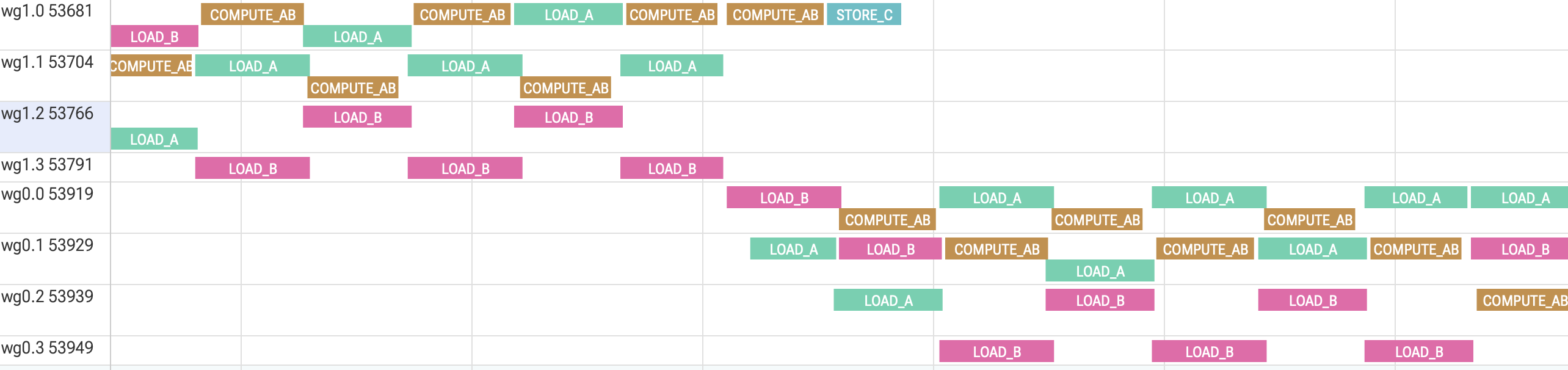
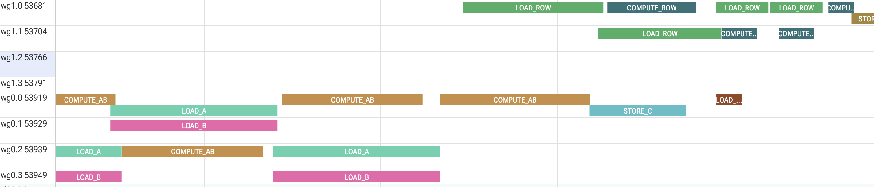
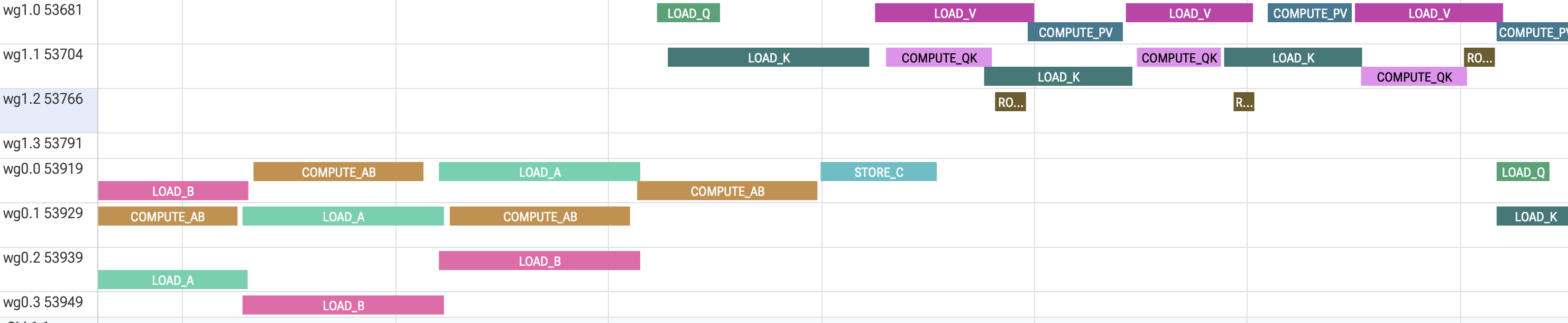
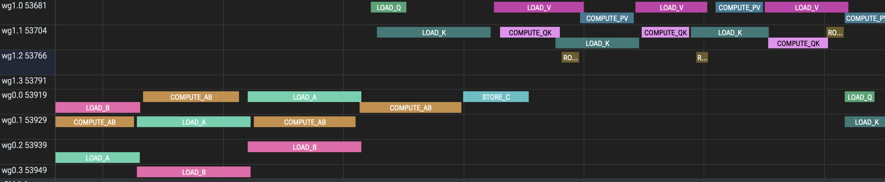
Intrakernel profiling is useful for visualizing asynchronous pipelines. Sample the per-SM %clock64 register and write the values to global memory as the kernel runs. Sample at the beginning and end of each pipeline stage, then export the data to a Perfetto trace. At the start of the kernel, also sample %globalTimer for synchronization because %clock64 is not necessarily synchronized across SMs. This is the overall per-SM visualization of the complete pipeline.

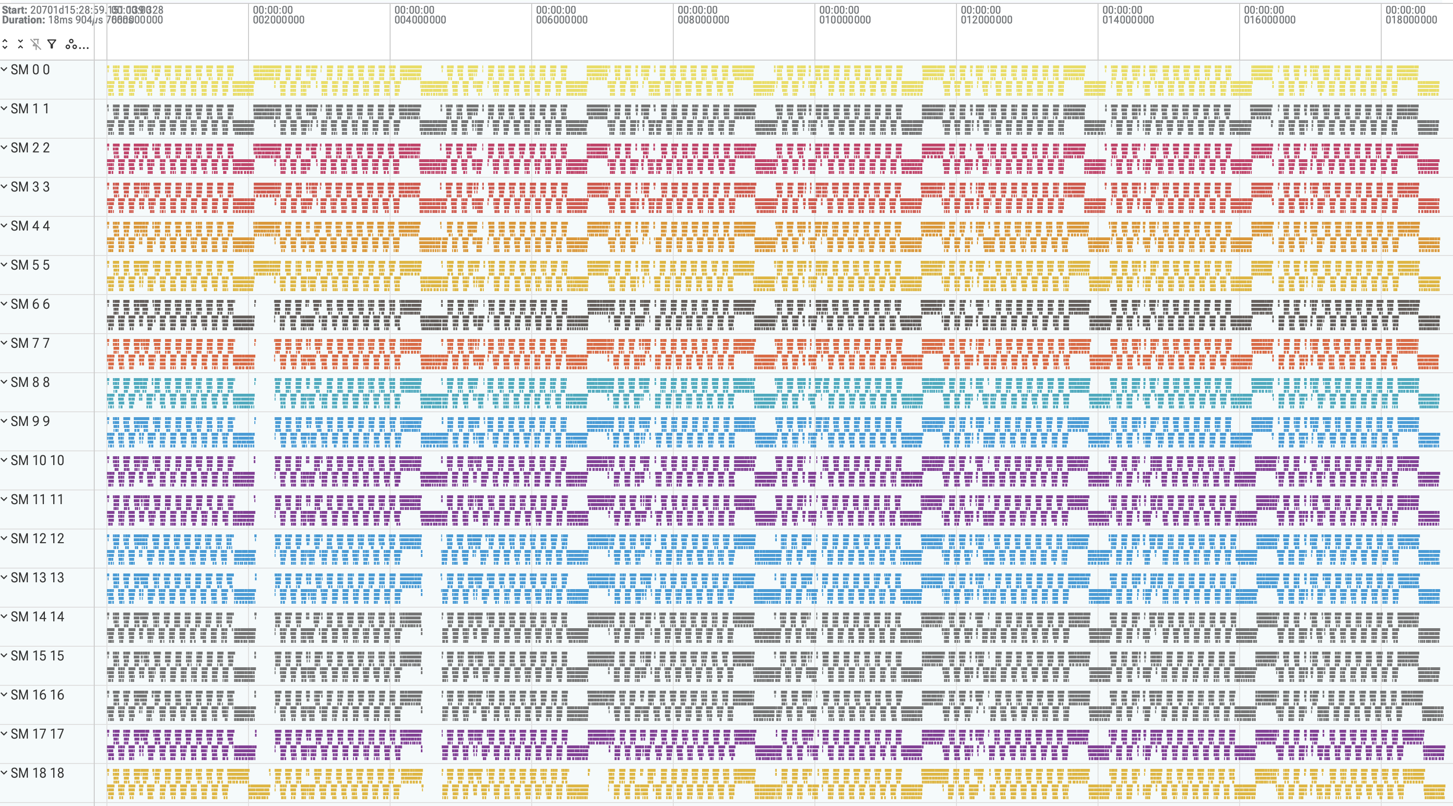
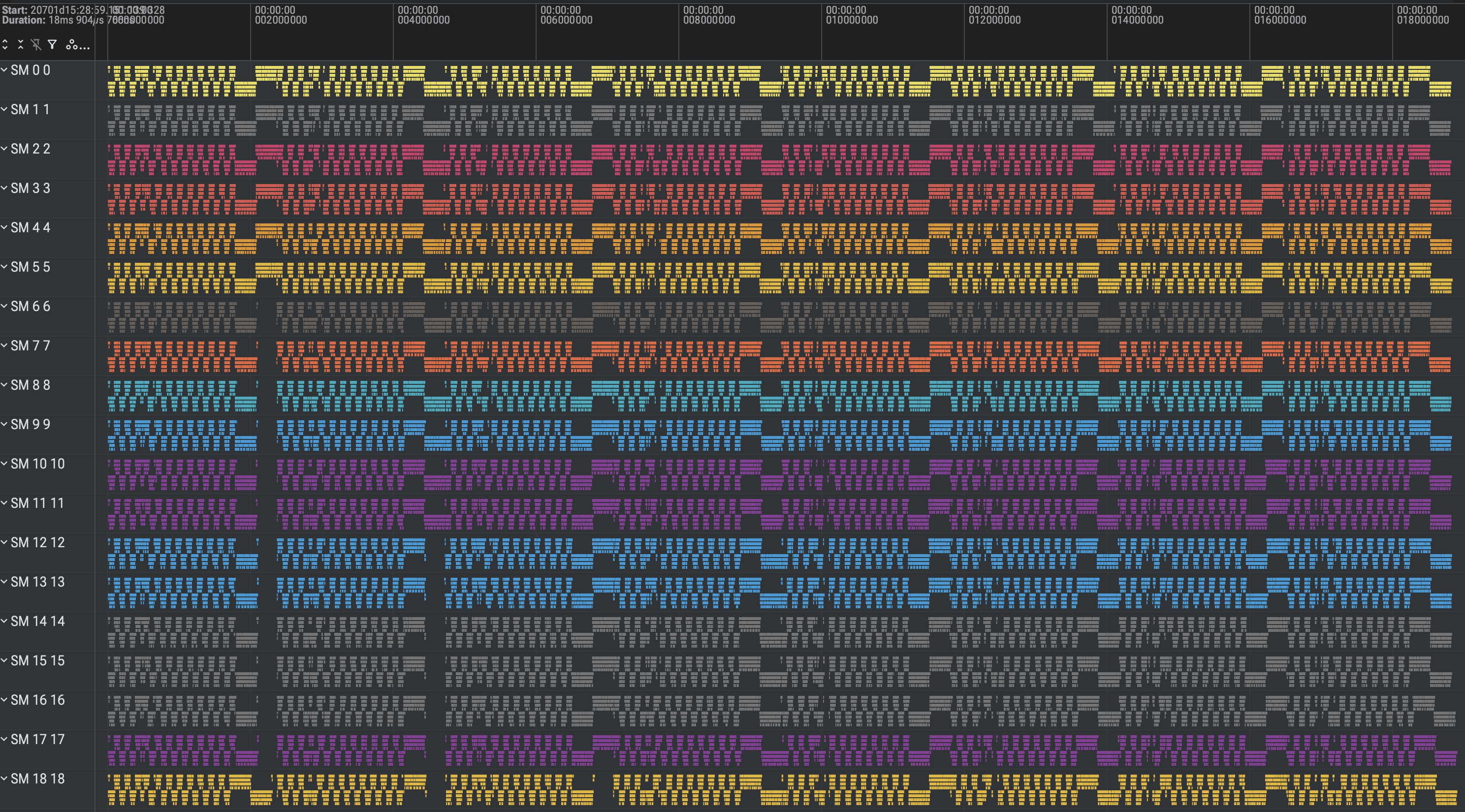
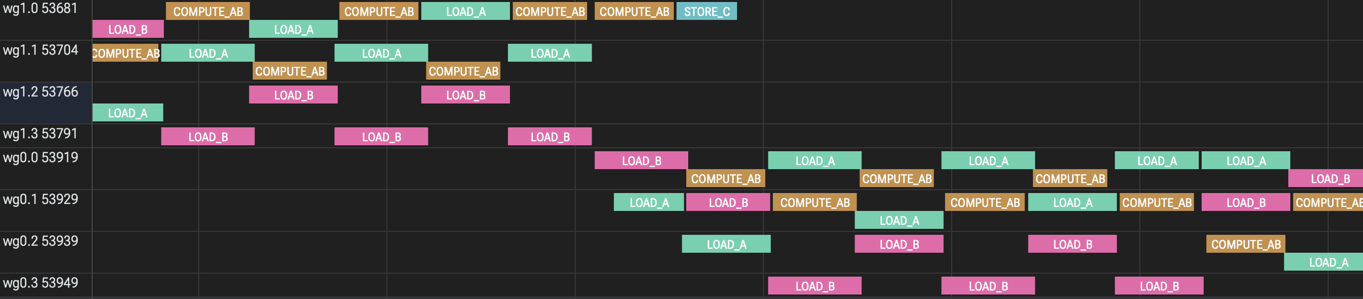
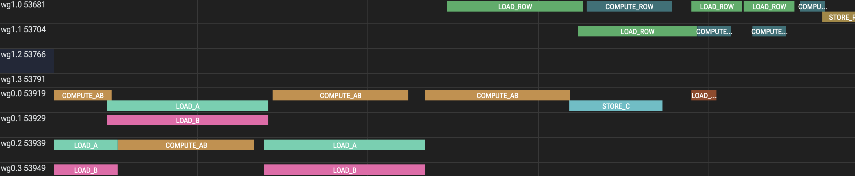
If we zoom at each pipeline you can clearly see how the load of the next pipeline work taken by the other warpgroup is overlapped with the work of the current warpgroup. We have almost eliminated load/store bubbles inter- and intra-operators and are working on compute!!

Matmul-Matmul Handoff

Matmul-RMSNorm Handoff

Matmul-Attention Handoff

Benchmarking

Three sweeps against torch.compile (inductor), torch.compile (TensorRT) and eager, on an RTX 5070 Ti locally and an RTX PRO 6000 rented from Modal. All numbers are TFLOP/s, higher is better.

Sequence length

embed_dim=1024, num_layers=8, 8 heads.

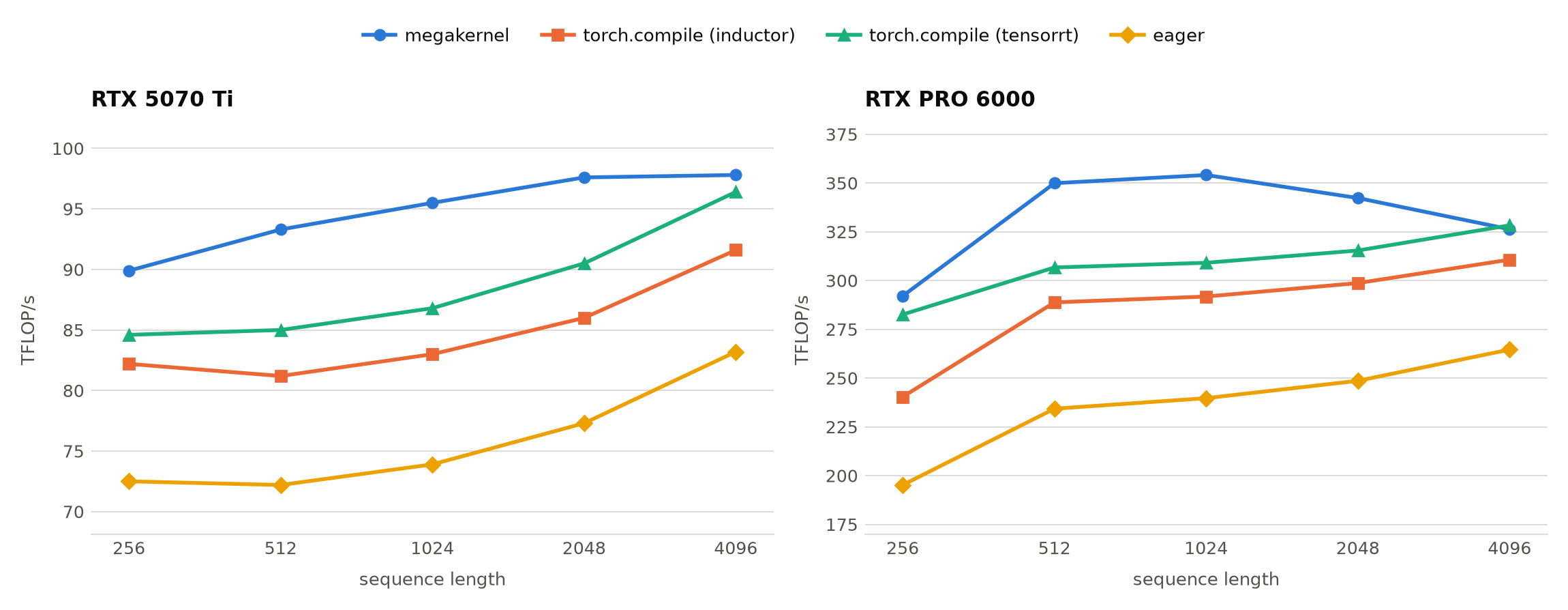
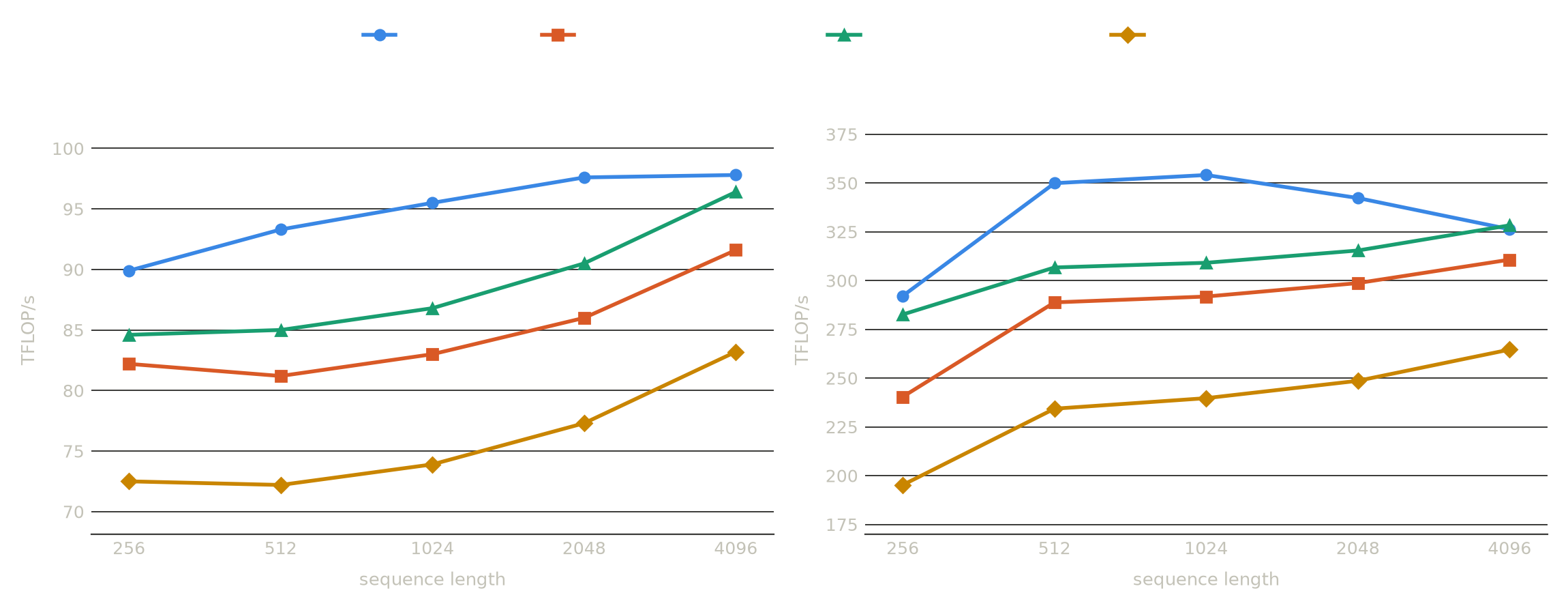
The lead over TensorRT peaks in the middle of the sweep (+10% at seq=1024 on the 5070 Ti, +15% on the PRO 6000) and collapses at the long end, where TensorRT actually edges ahead by 0.6% at seq=4096 on the PRO 6000.

Number of layers

embed_dim=1024, q_len=256, 8 heads.

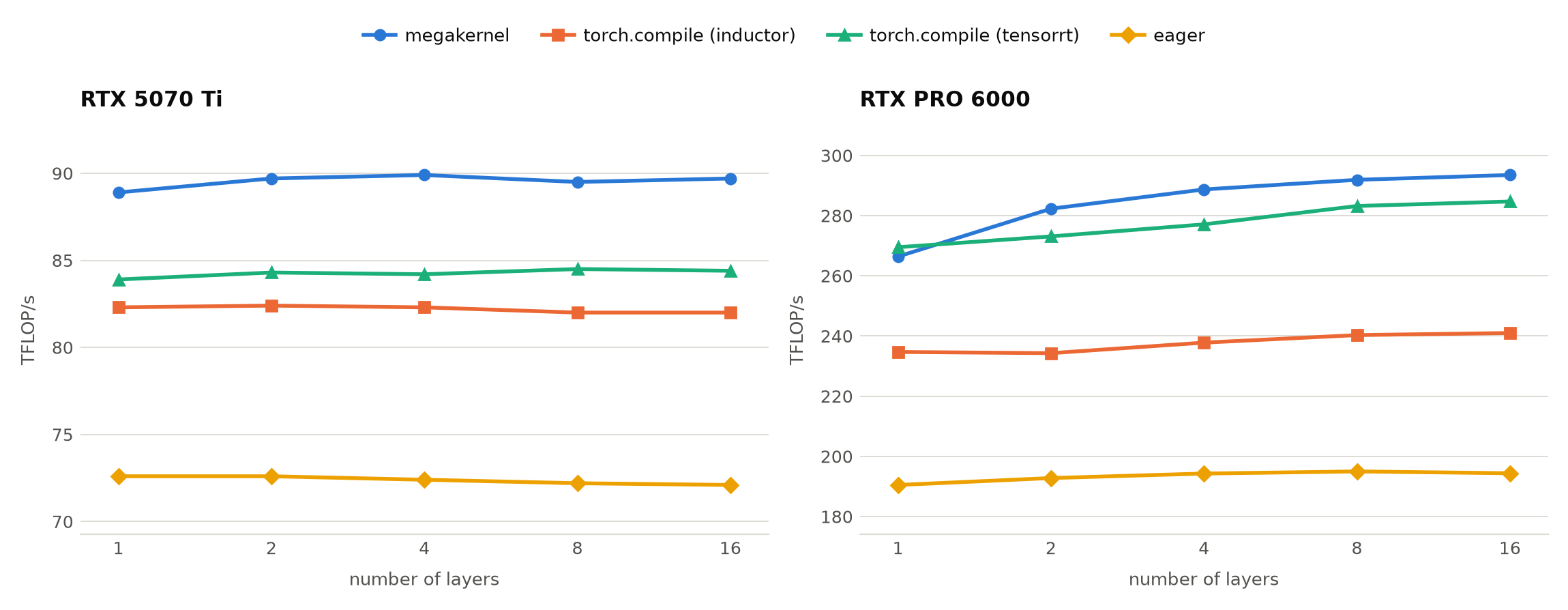
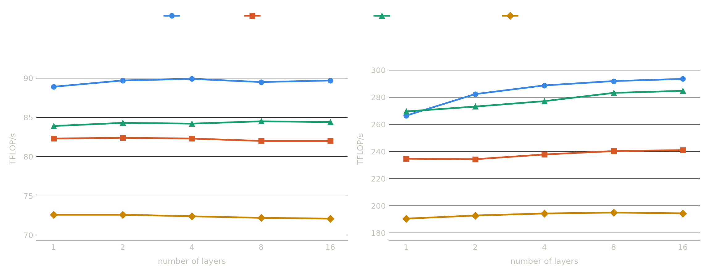
Flat in depth for every backend, so per-layer cost stays constant. The one loss is layers=1 on the PRO 6000 (266.4 vs 269.5). From two layers on it leads by 3-4%.

Embedding width and number of heads

1 layer, bs=8, q_len=256, head_dim=128 fixed.

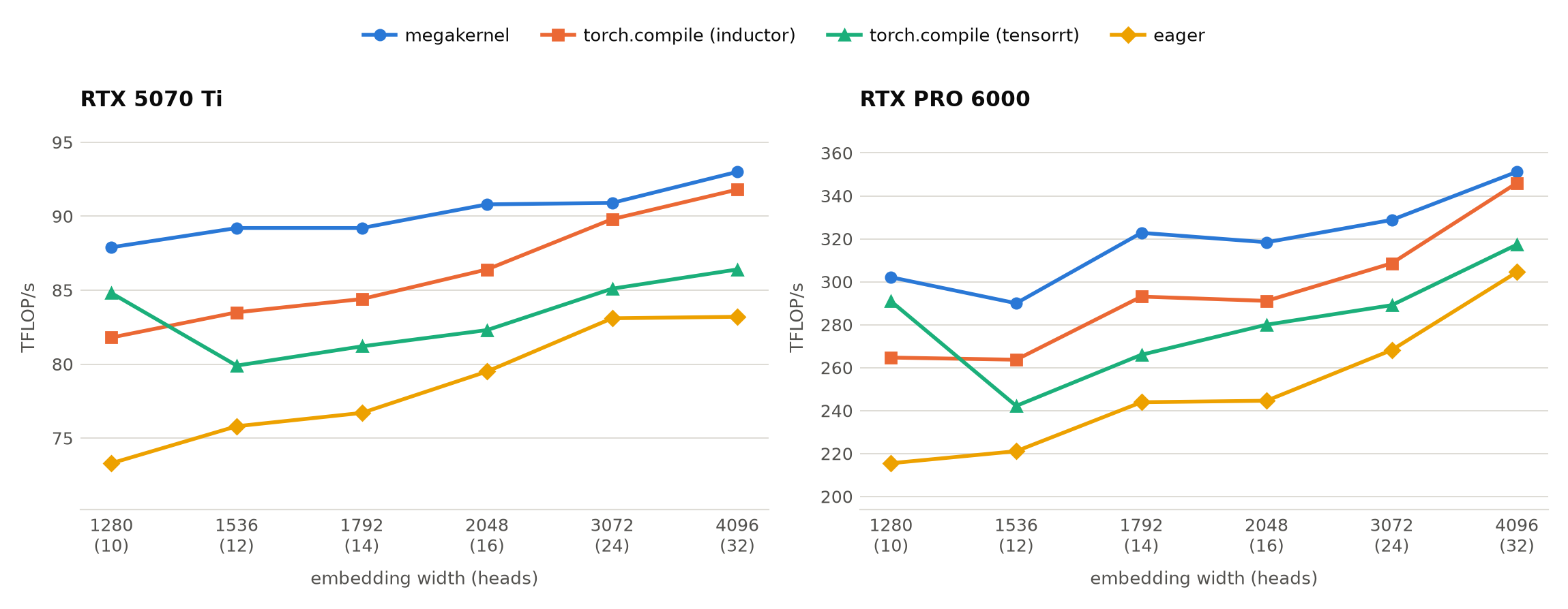
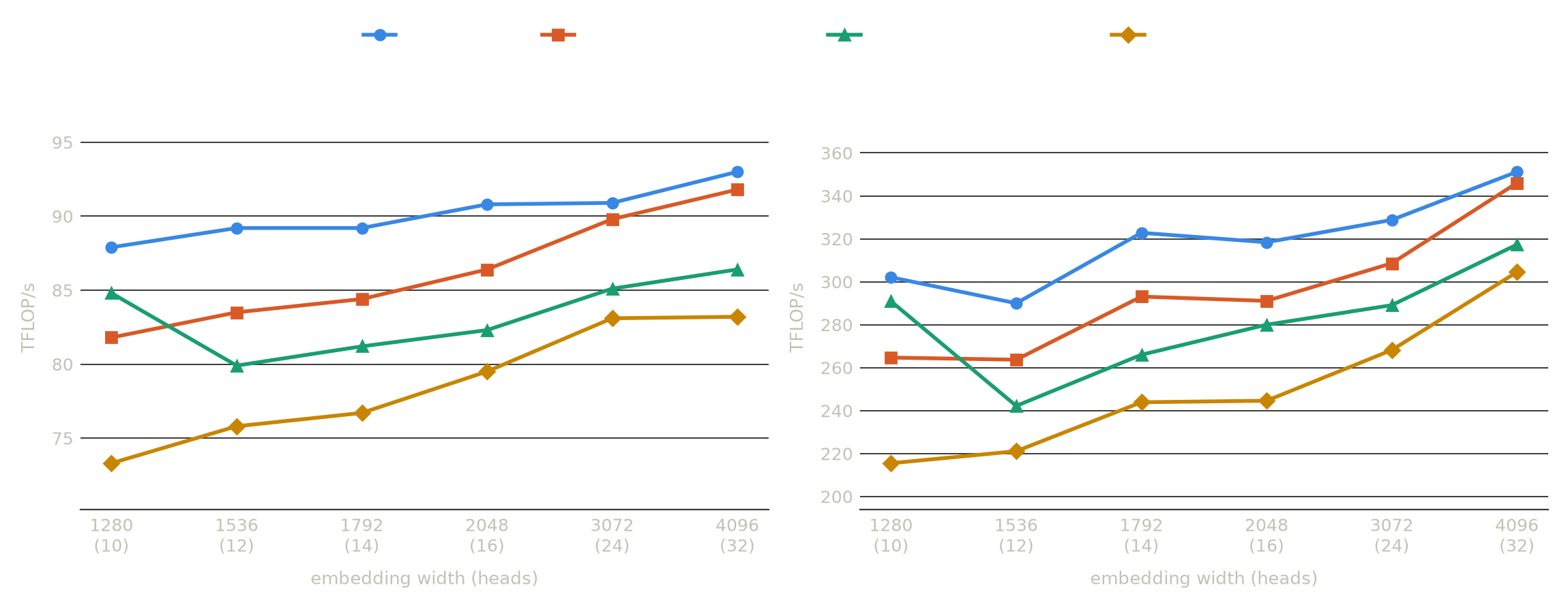
Same story on a different axis: +7.5% over inductor at embed_dim=1280 on the 5070 Ti and +14% on the PRO 6000, shrinking to +1.3% and +1.5% by embed_dim=4096 as each matmul gets large enough to saturate the tensor cores on its own.

Takeaways

The megakernel is fastest in all 16 configs on the 5070 Ti and in 14 of 16 on the PRO 6000, losing only at seq=4096 and layers=1 and by under 1.5% in both. The margin over eager is 9-29% on the 5070 Ti and 15-51% on the PRO 6000. It is largest exactly where per-op overhead would otherwise dominate and narrows as the workload becomes compute bound which is expected as the kernel does not make the tensor cores faster, it removes the launch and memory-roundtrip cost that torch.compile and eager still pay between every operator.

Next Up

The code for all of the above can be found on github.com/Parth-Badgujar/transformer-megakernel. This was a make shift implementation which cannot be used for actual LLM ops, I am currently working on a decode only megakernel for the latest architectures which also have linear attention and mixture-of-experts.

References

1. Modal. “GPU Glossary.” Modal. https://modal.com/gpu-glossary
2. Yifan Yang. “CuTe Copy.” Yifan Yang’s Blog. https://yang-yifan.github.io/blogs/cute_copy/cute_copy.html
3. Benjamin Spector, Jordan Juravsky, Stuart Sul, Owen Dugan, Dylan Lim, Dan Fu, Simran Arora, and Chris Ré. “Look Ma, No Bubbles! Designing a Low-Latency Megakernel for Llama-1B.” Hazy Research, May 27, 2025. https://hazyresearch.stanford.edu/blog/2025-05-27-no-bubbles
4. Thien Tran (gau-nernst). “Using TMA in CuteDSL.” gau-nernst’s blog, May 25, 2026. https://gau-nernst.github.io/cutedsl-tma/
5. Simon Veitner. simons blog. https://veitner.bearblog.dev/blog/
6. Lei Mao. Lei Mao’s Log Book. https://leimao.github.io/blog/
7. NVIDIA. “Parallel Thread Execution ISA Version 9.1.” NVIDIA CUDA Toolkit Documentation (archive 13.1.2). https://docs.nvidia.com/cuda/archive/13.1.2/parallel-thread-execution/contents.html
8. luongthecong123. “learn-cutedsl: Step-by-Step GEMM Optimization, One Hardware Feature at a Time.” GitHub. https://github.com/luongthecong123/learn-cutedsl
9. Colfax Research. Colfax International. https://research.colfax-intl.com
10. GPU MODE. “Getting Started with CuTe DSL.” YouTube. https://www.youtube.com/live/zHlz6mrdlZE